31 Feature Engineering
Feature engineering is a fancy machine learning way of saying “prepare your data for analysis”. But it’s also more than just getting your data in the right format. It’s about transforming variables to help the model provide more stable predictions – for example, encoding, modeling, or omitting missing data; creating new variables from the available dataset; and otherwise helping improve the model performance through transformations and modifications to the existing data before analysis.
One of the biggest challenges with feature engineering is what’s referred to as data leakage, which occurs when information from the test dataset leaks into the training dataset. Consider the simple example of normalizing or standardizing a variable (subtracting the variable mean from each value and then dividing by the standard deviation). Normalizing your variables is necessary for a wide range of predictive models, including any model using regularization methods, principal components analysis, and \(k\)-nearest neighbor models, among others. But when we normalize the variable, it is critical we do so relative to the training set, not relative to the full dataset. If we normalize the numeric variables in our full dataset and then divide it into test and training datasets, information from the test dataset has leaked into the training dataset. This seems simple enough - just wait to standardize until after splitting - but it becomes more complicated when we consider tuning a model. If we use a process like \(k\)-fold cross-validation, then we have to normalize within each fold to get an accurate representation of out-of-sample predictive accuracy.
In this chapter, we’ll introduce feature engineering using the {recipes} package from the {tidymodels} suite of packages which, as we will see, helps you to be explicit about the decisions you’re making, while avoiding potential issues with data leakage.
31.1 Basics of {recipes}
![]()
The {recipes} package is designed to replace the stats::model.matrix() function that you might be familiar with. For example, if you fit a model like the one below
##
## Call:
## lm(formula = bill_length_mm ~ species, data = penguins)
##
## Residuals:
##     Min      1Q  Median      3Q     Max
## -7.9338 -2.2049  0.0086  2.0662 12.0951
##
## Coefficients:
##                  Estimate Std. Error t value Pr(>|t|)
## (Intercept)       38.7914     0.2409  161.05   <2e-16 ***
## speciesChinstrap  10.0424     0.4323   23.23   <2e-16 ***
## speciesGentoo      8.7135     0.3595   24.24   <2e-16 ***
## ---
## Signif. codes:  0 '***' 0.001 '**' 0.01 '*' 0.05 '.' 0.1 ' ' 1
##
## Residual standard error: 2.96 on 339 degrees of freedom
##   (2 observations deleted due to missingness)
## Multiple R-squared:  0.7078, Adjusted R-squared:  0.7061
## F-statistic: 410.6 on 2 and 339 DF,  p-value: < 2.2e-16
You can see that our species column, which has the values Adelie, Gentoo, Chinstrap, is automatically dummy-coded for us, with the first level in the factor variable (Adelie) set as the reference group. The {recipes} package forces you to be a bit more explicit in these decisions. But it also has a much wider range of modifications it can make to the data.
Using {recipes} also allows you to more easily separate the pre-processing and modeling stages of your data analysis workflow. In the above example, you may not have even realized stats::model.matrix() was doing anything for you because it’s wrapped within the stats::lm() modeling code. But with {recipes}, you make the modifications to your data first and then conduct your analysis.
How does this separation work? With {recipes}, you can create a blueprint (or recipe) to apply to a given dataset, without actually applying those operations. You can then use this blueprint iteratively across sets of data (e.g., folds) as well as on new (potentially unseen) data that has the same structure (variables). This process helps avoid data leakage because all operations are carried forward and applied together, and no operations are conducted until explicitly requested.
31.2 Creating a recipe
Let’s read in some data and begin creating a basic recipe. We’ll work with the simulated statewide testing data introduced previously. This is a fairly decent sized dataset, and since we’re just illustrating concepts here, we’ll pull a random sample of 2% of the total data to make everything run a bit quicker. We’ll also remove the classification variable, which is just a categorical version of score, our outcome.
In the chunk below, we read in the data, sample a random 2% of the data (being careful to set a seed first so our results are reproducible), split it into training and test sets, and extract just the training dataset. We’ll hold off on splitting it into CV folds for now.
library(tidyverse)
library(tidymodels)

set.seed(8675309)
full_train <- read_csv("https://github.com/uo-datasci-specialization/c4-ml-fall-2020/raw/master/data/train.csv") %>%
  slice_sample(prop = 0.02) %>%
  select(-classification)

splt <- initial_split(full_train)
train <- training(splt)
A quick reminder, the data look like this
And you can see the full data dictionary on the Kaggle website here.
When creating recipes, we can still use the formula interface to define how the data will be modeled. In this case, we’ll say that the score column is predicted by everything else in the data frame.
Notice that I still declare the dataset (in this case, the training data), even though this is just a blueprint. It uses the dataset I provide to get the names of the columns, but it doesn’t actually do anything with this dataset (unless we ask it to). Let’s look at what this recipe looks like.
## Data Recipe
##
## Inputs:
##
##       role #variables
##    outcome          1
##  predictor         38
Notice it just states that this is a data recipe in which we have specified 1 outcome variable and 38 predictors.
We can prep this recipe to learn more.
## Data Recipe
##
## Inputs:
##
##       role #variables
##    outcome          1
##  predictor         38
##
## Training data contained 2841 data points and 2841 incomplete rows.
Notice we now get an additional message about how many rows are in the data, and how many of these rows contain missing (incomplete data). So the recipe is the blueprint, and we prep the recipe to get it to actually go into the data and conduct the operations. The dataset it has now, however, is just a placeholder than can be substituted in for any other dataset with an equivalent structure.
But of course, modeling score as the outcome with everything else predicting it is not a reasonable choice in this case. For example, we have many ID variables, and we also have multiple categorical variables. For some methods (like tree-based models) it might be okay to leave these categorical variables as they are, but for others (like any model in the linear regression family) we’ll want to encode them somehow (e.g., dummy code).
We can address these concerns by adding steps to our recipe. In the first step, we’ll update the role of all the ID variables so they are not included among the predictors. In the second, we will dummy code all nominal (i.e. categorical) variables.
rec <- recipe(score ~ ., train) %>%
  update_role(contains("id"), ncessch, new_role = "id vars") %>%
  step_dummy(all_nominal())
When updating the roles, we can change the variable label (text passed to the new_role argument) to be anything we want, so long as it’s not "predictor" or "outcome".
Notice in the above I am also using helper functions to apply the operations to all variables of a specific type. There are five main helper functions for creating recipes: all_predictors(), all_outcomes(), all_nominal(), all_numeric() and has_role(). You can use these together, including with negation (e.g., -all_outcomes() to specify the operation should not apply to the outcome variable(s)) to select any set of variables you want to apply the operation to.
Let’s try to prep this updated recipe.
## Error: Only one factor level in lang_cdUh oh! We have an error. Our recipe is trying to dummy code the lang_cd variable, but it has only one level. It’s kind of hard to dummy-code a constant!
Luckily, we can expand our recipe to first remove any zero-variance predictors, like so:
rec <- recipe(score ~ ., train) %>%
  update_role(contains("id"), ncessch, new_role = "id vars") %>%
  step_zv(all_predictors()) %>%
  step_dummy(all_nominal())
The _zv part stands for “zero variance” and should take care of this problem. Let’s try again.
## Data Recipe
##
## Inputs:
##
##       role #variables
##    id vars          6
##    outcome          1
##  predictor         32
##
## Training data contained 2841 data points and 2841 incomplete rows.
##
## Operations:
##
## Zero variance filter removed calc_admn_cd, lang_cd [trained]
## Dummy variables from gndr, ethnic_cd, tst_bnch, tst_dt, ... [trained]
Beautiful! Note we do still get a warning here, but I’ve omitted it in the text (we’ll come back to this in the section on Missing data). Our recipe says we now have 6 ID variables, 1 outcome, and 32 predictors, with 2841 data points (rows of data). The calc_admn_cd and lang_cd variables have been removed because they have zero variance, and several variables have been dummy coded, including gndr and ethnic_cd, among others.
Let’s dig just a bit deeper here though. What’s going on with these zero-variance variables? Let’s look back at the training data.
## # A tibble: 1 x 2
##   calc_admn_cd     n
##   <lgl>        <int>
## 1 NA 2841## # A tibble: 2 x 2
## lang_cd n
## <chr> <int>
## 1 S 80
## 2 <NA> 2761So at least in our sample, calc_admn_cd really is just fully missing, which means it might as well be dropped because it’s providing us exactly nothing. But that’s not the case with lang_cd. It has two values, NA and "S" (for “Spanish”). This variable represents the language the test was administered in and the NA values are actually meaningful here because they are the the “default” administration, meaning English. So rather than dropping these, let’s mutate them to transform the NA values to "E" for English. We could reasonably do this inside or outside the recipe, but a good rule of thumb is, if it can go in the recipe, put it in the recipe. It can’t hurt, and doing operations outside of the recipe risks data leakage.
rec <- recipe(score ~ ., train) %>%
  update_role(contains("id"), ncessch, new_role = "id vars") %>%
  step_mutate(lang_cd = ifelse(is.na(lang_cd), "E", lang_cd)) %>%
  step_zv(all_predictors()) %>%
  step_dummy(all_nominal())
Let’s take a look at what our data would actually look like when applying this recipe now. First, we’ll prep the recipe
## Data Recipe
##
## Inputs:
##
##       role #variables
##    id vars          6
##    outcome          1
##  predictor         32
##
## Training data contained 2841 data points and 2841 incomplete rows.
##
## Operations:
##
## Variable mutation for lang_cd [trained]
## Zero variance filter removed calc_admn_cd [trained]
## Dummy variables from gndr, ethnic_cd, tst_bnch, tst_dt, ... [trained]
And we see that lang_cd is no longer being caught by the zero variance filter. Next we’ll bake the prepped recipe to actually apply it to our data. If we specify new_data = NULL, bake() will apply the operation to the data we originally specified in the recipe. But we can also pass new data as an additional argument and it will apply the operations to that data instead of the data specified in the recipe.
## # A tibble: 2,841 x 106
##        id attnd_dist_inst… attnd_schl_inst… enrl_grd partic_dist_ins…
##     <dbl>            <dbl>            <dbl>    <dbl>            <dbl>
##  1  62576             2083             1353        7             2083
##  2  71424             2180              878        6             2180
##  3 179893             2244             1334        3             2244
##  4 136083             2142             4858        5             2142
##  5 196809             2212             1068        3             2212
##  6  13931             2088              581        8             2088
##  7 103344             1926              102        6             1926
##  8 105122             2142              766        6             2142
##  9 172543             1965              197        4             1965
## 10  45153             2083              542        6             2083
## # … with 2,831 more rows, and 101 more variables: partic_schl_inst_id <dbl>,
## #   lang_cd <fct>, ncessch <dbl>, lat <dbl>, lon <dbl>, score <dbl>,
## #   gndr_M <dbl>, ethnic_cd_B <dbl>, ethnic_cd_H <dbl>, ethnic_cd_I <dbl>,
## #   ethnic_cd_M <dbl>, ethnic_cd_P <dbl>, ethnic_cd_W <dbl>,
## #   tst_bnch_X2B <dbl>, tst_bnch_X3B <dbl>, tst_bnch_G4 <dbl>,
## #   tst_bnch_G6 <dbl>, tst_bnch_G7 <dbl>, tst_dt_X3.21.2018.0.00.00 <dbl>,
## #   tst_dt_X3.22.2018.0.00.00 <dbl>, tst_dt_X3.23.2018.0.00.00 <dbl>,
## #   tst_dt_X3.8.2018.0.00.00 <dbl>, tst_dt_X3.9.2018.0.00.00 <dbl>,
## #   tst_dt_X4.10.2018.0.00.00 <dbl>, tst_dt_X4.11.2018.0.00.00 <dbl>,
## #   tst_dt_X4.12.2018.0.00.00 <dbl>, tst_dt_X4.13.2018.0.00.00 <dbl>,
## #   tst_dt_X4.16.2018.0.00.00 <dbl>, tst_dt_X4.17.2018.0.00.00 <dbl>,
## #   tst_dt_X4.18.2018.0.00.00 <dbl>, tst_dt_X4.19.2018.0.00.00 <dbl>,
## #   tst_dt_X4.2.2018.0.00.00 <dbl>, tst_dt_X4.20.2018.0.00.00 <dbl>,
## #   tst_dt_X4.23.2018.0.00.00 <dbl>, tst_dt_X4.24.2018.0.00.00 <dbl>,
## #   tst_dt_X4.25.2018.0.00.00 <dbl>, tst_dt_X4.26.2018.0.00.00 <dbl>,
## #   tst_dt_X4.27.2018.0.00.00 <dbl>, tst_dt_X4.30.2018.0.00.00 <dbl>,
## #   tst_dt_X4.5.2018.0.00.00 <dbl>, tst_dt_X4.6.2018.0.00.00 <dbl>,
## #   tst_dt_X4.9.2018.0.00.00 <dbl>, tst_dt_X5.1.2018.0.00.00 <dbl>,
## #   tst_dt_X5.10.2018.0.00.00 <dbl>, tst_dt_X5.11.2018.0.00.00 <dbl>,
## #   tst_dt_X5.14.2018.0.00.00 <dbl>, tst_dt_X5.15.2018.0.00.00 <dbl>,
## #   tst_dt_X5.16.2018.0.00.00 <dbl>, tst_dt_X5.17.2018.0.00.00 <dbl>,
## #   tst_dt_X5.18.2018.0.00.00 <dbl>, tst_dt_X5.2.2018.0.00.00 <dbl>,
## #   tst_dt_X5.21.2018.0.00.00 <dbl>, tst_dt_X5.22.2018.0.00.00 <dbl>,
## #   tst_dt_X5.23.2018.0.00.00 <dbl>, tst_dt_X5.24.2018.0.00.00 <dbl>,
## #   tst_dt_X5.25.2018.0.00.00 <dbl>, tst_dt_X5.29.2018.0.00.00 <dbl>,
## #   tst_dt_X5.3.2018.0.00.00 <dbl>, tst_dt_X5.30.2018.0.00.00 <dbl>,
## #   tst_dt_X5.31.2018.0.00.00 <dbl>, tst_dt_X5.4.2018.0.00.00 <dbl>,
## #   tst_dt_X5.7.2018.0.00.00 <dbl>, tst_dt_X5.8.2018.0.00.00 <dbl>,
## #   tst_dt_X5.9.2018.0.00.00 <dbl>, tst_dt_X6.1.2018.0.00.00 <dbl>,
## #   tst_dt_X6.4.2018.0.00.00 <dbl>, tst_dt_X6.5.2018.0.00.00 <dbl>,
## #   tst_dt_X6.6.2018.0.00.00 <dbl>, tst_dt_X6.7.2018.0.00.00 <dbl>,
## #   tst_dt_X6.8.2018.0.00.00 <dbl>, migrant_ed_fg_Y <dbl>, ind_ed_fg_Y <dbl>,
## #   sp_ed_fg_Y <dbl>, tag_ed_fg_Y <dbl>, econ_dsvntg_Y <dbl>, ayp_lep_B <dbl>,
## #   ayp_lep_E <dbl>, ayp_lep_F <dbl>, ayp_lep_M <dbl>, ayp_lep_N <dbl>,
## #   ayp_lep_S <dbl>, ayp_lep_W <dbl>, ayp_lep_X <dbl>, ayp_lep_Y <dbl>,
## #   stay_in_dist_Y <dbl>, stay_in_schl_Y <dbl>, dist_sped_Y <dbl>,
## #   trgt_assist_fg_Y <dbl>, ayp_dist_partic_Y <dbl>, ayp_schl_partic_Y <dbl>,
## #   ayp_dist_prfrm_Y <dbl>, ayp_schl_prfrm_Y <dbl>, rc_dist_partic_Y <dbl>,
## #   rc_schl_partic_Y <dbl>, rc_dist_prfrm_Y <dbl>, rc_schl_prfrm_Y <dbl>,
## #   tst_atmpt_fg_Y <dbl>, grp_rpt_dist_partic_Y <dbl>,
## #   grp_rpt_schl_partic_Y <dbl>, grp_rpt_dist_prfrm_Y <dbl>, …
And now we can actually see the dummy-coded categorical variables, along with the other operations we requested. For example, calc_admn_cd is not in the dataset. Notice the ID variables are output though, which makes sense because they are often neccessary for joining with other data sources. But it’s important to realize that they are output (i.e., all variables are returned, regardless of role) because if we passed this directly to a model they would be included as predictors. Note that there may be reasons you would want to include a school and/or district level ID variable in your modeling, but you certainly would not want redundant variables.
We do still have one minor issue with this recipe though, which is pretty evident when looking at the column names of our baked dataset. The tst_dt variable, which specifies the date the test was taken, was treated as a categorical variable because it was read in as a character vector. That means all the dates are being dummy coded! Let’s fix this by just transforming it to a date within our step_mutate.
rec <- recipe(score ~ ., train) %>%
  update_role(contains("id"), ncessch, new_role = "id vars") %>%
  step_mutate(lang_cd = factor(ifelse(is.na(lang_cd), "E", lang_cd)),
              tst_dt = lubridate::mdy_hms(tst_dt)) %>%
  step_zv(all_predictors()) %>%
  step_dummy(all_nominal())
And now when we prep/bake the dataset it’s still a date variable, which is what we probably want (it will be modeled as a numeric variable).
## # A tibble: 2,841 x 55
##        id attnd_dist_inst… attnd_schl_inst… enrl_grd tst_dt
##     <dbl>            <dbl>            <dbl>    <dbl> <dttm>
##  1  62576             2083             1353        7 2018-05-16 00:00:00
##  2  71424             2180              878        6 2018-04-24 00:00:00
##  3 179893             2244             1334        3 2018-05-25 00:00:00
##  4 136083             2142             4858        5 2018-05-24 00:00:00
##  5 196809             2212             1068        3 2018-05-16 00:00:00
##  6  13931             2088              581        8 2018-06-06 00:00:00
##  7 103344             1926              102        6 2018-06-04 00:00:00
##  8 105122             2142              766        6 2018-05-08 00:00:00
##  9 172543             1965              197        4 2018-05-23 00:00:00
## 10  45153             2083              542        6 2018-05-10 00:00:00
## # … with 2,831 more rows, and 50 more variables: partic_dist_inst_id <dbl>,
## #   partic_schl_inst_id <dbl>, ncessch <dbl>, lat <dbl>, lon <dbl>,
## #   score <dbl>, gndr_M <dbl>, ethnic_cd_B <dbl>, ethnic_cd_H <dbl>,
## #   ethnic_cd_I <dbl>, ethnic_cd_M <dbl>, ethnic_cd_P <dbl>, ethnic_cd_W <dbl>,
## #   tst_bnch_X2B <dbl>, tst_bnch_X3B <dbl>, tst_bnch_G4 <dbl>,
## #   tst_bnch_G6 <dbl>, tst_bnch_G7 <dbl>, migrant_ed_fg_Y <dbl>,
## #   ind_ed_fg_Y <dbl>, sp_ed_fg_Y <dbl>, tag_ed_fg_Y <dbl>,
## #   econ_dsvntg_Y <dbl>, ayp_lep_B <dbl>, ayp_lep_E <dbl>, ayp_lep_F <dbl>,
## #   ayp_lep_M <dbl>, ayp_lep_N <dbl>, ayp_lep_S <dbl>, ayp_lep_W <dbl>,
## #   ayp_lep_X <dbl>, ayp_lep_Y <dbl>, stay_in_dist_Y <dbl>,
## #   stay_in_schl_Y <dbl>, dist_sped_Y <dbl>, trgt_assist_fg_Y <dbl>,
## #   ayp_dist_partic_Y <dbl>, ayp_schl_partic_Y <dbl>, ayp_dist_prfrm_Y <dbl>,
## #   ayp_schl_prfrm_Y <dbl>, rc_dist_partic_Y <dbl>, rc_schl_partic_Y <dbl>,
## #   rc_dist_prfrm_Y <dbl>, rc_schl_prfrm_Y <dbl>, lang_cd_E <dbl>,
## #   tst_atmpt_fg_Y <dbl>, grp_rpt_dist_partic_Y <dbl>,
## #   grp_rpt_schl_partic_Y <dbl>, grp_rpt_dist_prfrm_Y <dbl>,
## #   grp_rpt_schl_prfrm_Y <dbl>
31.2.1 Order matters
It’s important to realize that the order of the steps matters. In our recipe, we first declare ID variables as having a different role than predictors or outcomes. We then modify two variables, remove zero-variance predictors, and finally dummy code all categorical (nominal) variables. What happens if we instead dummy code and then remove zero-variance predictors?
rec <- recipe(score ~ ., train) %>%
  step_dummy(all_nominal()) %>%
  step_zv(all_predictors())

prep(rec)
## Error: Only one factor level in lang_cdWe end up with our original error. We don’t get this error if we remove zero variance predictors and then dummy code.
rec <- recipe(score ~ ., train) %>%
  step_zv(all_predictors()) %>%
  step_dummy(all_nominal())

prep(rec)
## Data Recipe
##
## Inputs:
##
## role #variables
## outcome 1
## predictor 38
##
## Training data contained 2841 data points and 2841 incomplete rows.
##
## Operations:
##
## Zero variance filter removed calc_admn_cd, lang_cd [trained]
## Dummy variables from gndr, ethnic_cd, tst_bnch, tst_dt, ... [trained]The fact that order matters may occasionally require that you apply the same operation at multiple steps (e.g., a near zero variance filter could be applied before and after dummy-coding).
All of the above serves as a basic introduction to developing a recipe, and what follows goes into more detail on specific feature engineering pieces. For complete information on all possible recipe steps, please see the documentation.
31.3 Encoding categorical data
For many (but not all) modeling frameworks, categorical data must be transformed somehow. The most common strategy for this is dummy coding, which stats::model.matrix() will do for you automatically using the stats::contrasts() function. There are also other coding schemes you can use with base R, such as Helmert and polynomial coding (see ?contrasts and related functions). Dummy coding leaves one group out (the first level of the factor, by default) and creates new columns for all the other groups coded \(0\) or \(1\) depending on whether the original variable represented that value or not. For example:
##       green red
## blue      0   0
## green     1   0
## red       0   1
In the above, "blue" has been assigned as the reference category (note that factor levels are assigned in alphabetical order by default), and dummy variables have been created for "green" and "red". In a linear regression framework, "blue" would become the intercept.
We can recreate this same coding scheme with {recipes}, but we need to first put it in a data frame.
##       f      score
## 1   red  1.0734291
## 2   red -0.2675359
## 3  blue  0.7512238
## 4 green  0.5436071
## 5 green  0.6940371
## 6 green -0.6446104## # A tibble: 6 x 3
## score f_green f_red
## <dbl> <dbl> <dbl>
## 1 1.07 0 1
## 2 -0.268 0 1
## 3 0.751 0 0
## 4 0.544 1 0
## 5 0.694 1 0
## 6 -0.645 1 0In the above, we’ve created the actual columns we need, while in the base example we only created the contrast matrix (although it’s relatively straightforward to then create the columns).
The {recipes} version is, admittedly, a fair amount of additional code, but as we saw in the previous section, {recipes} is capable of making a wide range of transformation in a systematic way.
31.3.1 Transformations beyond dummy coding
Although less used in inferential statistics, there are a number of additional transformations we can use to encode categorical data. The most straightforward is one-hot encoding. One-hot encoding is essentially equivalent to dummy coding except we create the variables for all levels in the categorical variable (i.e., we do not leave one out as a reference group). This generally makes them less useful in linear regression frameworks (unless the model intercept is dropped), but they can be highly useful in a number of other frameworks, such as tree-based methods (covered later in the book).
To use one-hot encoding, we pass the additional one_hot argument to step_dummy().
## # A tibble: 6 x 4
##    score f_blue f_green f_red
##    <dbl>  <dbl>   <dbl> <dbl>
## 1  1.07       0       0     1
## 2 -0.268      0       0     1
## 3  0.751      1       0     0
## 4  0.544      0       1     0
## 5  0.694      0       1     0
## 6 -0.645      0       1     0
Another relatively common encoding scheme, particularly within natural language processing frameworks, is integer encoding, where each level is associated with a unique integer. For example
## # A tibble: 6 x 2
##       f  score
##   <dbl>  <dbl>
## 1     3  1.07
## 2     3 -0.268
## 3     1  0.751
## 4     2  0.544
## 5     2  0.694
## 6     2 -0.645
Notice that the syntax is essentially equivalent to the previous dummy-coding example, but we’ve just swapped out step_dummy() for step_integer(). Integer encoding can be useful in natural language processing in particular because words can be encoded as integers, and then the algorithm can search for patterns in the numbers.
31.3.2 Handling new levels
One other very common problem with encoding categorical data is how to handle new, unseen levels. For example, let’s take a look at the recipe below:
We will have no problem creating dummy variables within this recipe as long as the levels of \(f\) are within those contained in df$f (or, more mathematically, where \(f \in F\)). But what if, in a new sample, \(f =\) “purple” or \(f =\) “gray”? Let’s try and see what happens.
df2 <- data.frame(f = factor(c("blue", "green", "purple", "gray")),
                  score = rnorm(4))
rec %>%
  prep() %>%
  bake(new_data = df2)
## # A tibble: 4 x 3
## score f_green f_red
## <dbl> <dbl> <dbl>
## 1 1.39 0 0
## 2 0.616 1 0
## 3 -2.35 NA NA
## 4 -0.165 NA NAWe end up propagating missing data, which is obviously less than ideal. Luckily, the solution is pretty straightforward. We just add a new step to our recipe to handle novel (or new) categories, lumping them all in their own level (labeled with the suffix _new).
rec <- recipe(score ~ f, data = df) %>%
  step_novel(f) %>%
  step_dummy(f)

rec %>%
  prep() %>%
  bake(new_data = df2)
## # A tibble: 4 x 4
## score f_green f_red f_new
## <dbl> <dbl> <dbl> <dbl>
## 1 1.39 0 0 0
## 2 0.616 1 0 0
## 3 -2.35 0 0 1
## 4 -0.165 0 0 1This is not perfect, because "purple" and "orange" may be highly different, and we’re modeling them as a single category. But at least we’re able to move forward with our model without introducing new missing data. As an aside, this is a small example of why having good training data is so important. If you don’t have all the levels of a categorical variable represented, you may end up essentially collapsing levels when there is meaningful variance that could be parsed out.
You can also use a similar approach with step_other() if you have a categorical variable with lots of levels (and a small-ish \(n\) by comparison). Using step_other(), you specify a threshold below which levels should be collapsed into a single “other” category. The threshold can be passed as a proportion or a frequency.
31.3.3 Final thoughts on encoding categorical data
There are, of course, many other ways you can encode categorical data. One important consideration is whether or not the variable is ordered (e.g., low, medium, high) in which case it may make sense to have a corresponding ordered numeric variable (e.g., \(0\), \(1\), \(2\)). Of course, the method of coding these ordered values will relate to assumptions of your modeling process. For example, in the previous example, we assumed that there is a linear, constant change across categories. In our experience, however, the combination of dummy coding (with potentially a one-hot alternative used), integer coding, or simply leaving the categorical variables as they are (for specific frameworks, like tree-based methods) is sufficient most (but not all) of the time. For a more complete discussion of encoding categorical data for predictive modeling frameworks, we recommend Chapter 5 of Kuhn & Johnson (2019).
31.4 Dealing with low variance predictors
Occasionally you have (or can create) variables that are highly imbalanced. A common example might include a gender variable that takes on the values “male”, “female”, “non-binary”, “other”, and “refused to answer”. Once you dummy-code a variable like this, it is possible that one or more of the categories may be so infrequent that it makes modeling that category difficult. This is not to say that these categories are not important, particularly when considering the representation of your training dataset to real-world applications (and any demographic variable is going to be associated with issues of ethics). Ignoring this variation may lead to systematic biases in model predictions. However, you also regularly have to make compromises to get models to work and be useful. One of those compromises often includes (with many types of variables, not just demographics) dropping highly imbalanced predictors.
Let’s look back at our statewide testing data. Let’s bake the final recipe from our Creating a recipe section on the training data and look at the dummy variables that are created.
rec <- recipe(score ~ ., train) %>%
  update_role(contains("id"), ncessch, new_role = "id vars") %>%
  step_mutate(lang_cd = factor(ifelse(is.na(lang_cd), "E", lang_cd)),
              tst_dt = lubridate::mdy_hms(tst_dt)) %>%
  step_zv(all_predictors()) %>%
  step_dummy(all_nominal())

baked <- rec %>%
  prep() %>%
  bake(new_data = NULL)
Below is a table of just the categorical variables and the frequency of each value.
The relative frequency of many of these looks fine, but for some one category has very low frequency. For example, ayp_lep_M has 576 observations (from our random 2% sample) that were \(0\), and only 2 that were \(1\). This is the same for ayp_lep_S. We may therefore consider applying a near-zero variance filter to drop these columns. Let’s try this, and then we’ll talk a bit more about what the filter is actually doing.
rec_nzv <- rec %>%
  step_nzv(all_predictors())

baked_rm_nzv <- rec_nzv %>%
  prep() %>%
  bake(new_data = NULL)
Let’s look at what columns are in baked that were removed from baked_rm_nzv.
##  [1] "ethnic_cd_B"           "ethnic_cd_I"           "ethnic_cd_P"
##  [4] "migrant_ed_fg_Y"       "ind_ed_fg_Y"           "ayp_lep_B"
##  [7] "ayp_lep_M"             "ayp_lep_S"             "ayp_lep_W"
## [10] "stay_in_dist_Y"        "stay_in_schl_Y"        "dist_sped_Y"
## [13] "trgt_assist_fg_Y"      "ayp_dist_partic_Y"     "ayp_schl_partic_Y"
## [16] "ayp_dist_prfrm_Y"      "ayp_schl_prfrm_Y"      "rc_dist_partic_Y"
## [19] "rc_schl_partic_Y"      "rc_dist_prfrm_Y"       "rc_schl_prfrm_Y"
## [22] "lang_cd_E"             "tst_atmpt_fg_Y"        "grp_rpt_dist_partic_Y"
## [25] "grp_rpt_schl_partic_Y" "grp_rpt_dist_prfrm_Y"  "grp_rpt_schl_prfrm_Y"
As you can see, the near-zero variance filter has been quite aggressive here, removing 27 columns. Looking back at our table of variables, we can see that, for example, there are 55 students coded Black out of 2841, and it could be reasonably argued that this column is worth keeping in the model.
So how is step_nzv working and how can we adjust it to be not quite so aggressive? Variables are flagged for being near-zero variance if they
- Have very few unique values, and
- The frequency ratio for the most common value to the second most common value is large
These criteria are implemented in step_nzv through the unique_cut and freq_cut arguments, respectively. unique_cut is estimated as the number of unique values divided by the total number of samples (length of the column) times 100 (i.e., it is a percent). freq_cut is estimated by dividing the most common level frequency by the second most common level frequency. The default for unique_cut is \(10\), while the default for freq_cut is \(95/5 = 19\). For a column to be “caught” by a near-zero variance filter, and removed from the training set, it must be below the specified unique_cut and above the specified freq_cut.
In the case of ethnic_cd_B, we see that there are two unique values, \(0\) and \(1\) (because it’s a dummy-coded variable). There are 2841 rows, so the unique_cut value is \((2 / 2841) \times 100 = 0.07\). The frequency ratio is \(2786/55 = 50.65\). It therefore meets both of the default criteria (below unique_cut and above freq_cut) and is removed.
If you’re applying a near-zero variance filter on dummy variables, there will always be only 2 values, leading to a small unique_cut. This might encourage you to up the freq_cut to a higher value. Let’s try this approach
rec_nzv2 <- rec %>%
  step_nzv(all_predictors(),
           freq_cut = 99/1)

baked_rm_nzv2 <- rec_nzv2 %>%
  prep() %>%
  bake(new_data = NULL)

removed_columns2 <- names(baked)[!(names(baked) %in% names(baked_rm_nzv2))]
removed_columns2
## [1] "ethnic_cd_P" "ayp_lep_M" "ayp_lep_S"
## [4] "ayp_lep_W" "dist_sped_Y" "ayp_dist_partic_Y"
## [7] "ayp_schl_partic_Y" "rc_dist_partic_Y" "rc_schl_partic_Y"
## [10] "tst_atmpt_fg_Y" "grp_rpt_dist_partic_Y" "grp_rpt_schl_partic_Y"
## [13] "grp_rpt_dist_prfrm_Y"Removing near-zero variance dummy variables can be a bit tricky because they will essentially always meet the unique_cut criteria. But it can be achieved by fiddling with the freq_cut variable and, actually, could be considered part of your model tuning process. In this case, we’ve set it so variables will be removed if greater than 99 out of every 100 cases is the same. This led to only 13 variables being flagged and removed. But we could continue on even further specifying, for example, that 499 out of every 500 must be the same for the variable to be flagged. At some point, however, you’ll end up with variables that have such low variance that model estimation becomes difficult, which is the purpose of applying the near-zero variance filter in the first place.
31.5 Missing data
If we look closely at our statewide testing data, we will see that there is a considerable amount of missingness. In fact, every row of the data frame has at least one value that is missing. The amount to which missing data impacts your work varies by field, but in most fields you’re likely to run into situations where you have to handle missing data in some way. The purpose of this section is to discuss a few approaches using {recipes} to handle missingness for predictive modeling purposes. Note that this is not a comprehensive discussion on the topic (for which, we recommend Little and Rubin (2002)), but is instead an applied discussion of what you can do. As with many aspects of data analysis, generally, there is no single approach that will always work best, and it’s worth trying a few different approaches in your model development to see how different choices impact your model performance.
There are three basic ways of handling missing data:
- Omit rows of the data frame that include missing values
- Encode or Impute the missing data
- Ignore the missing data and estimate from the available data
The last option is not always feasible and will depend the modeling framework you’re working within. Some estimation procedures can also lend themselves to efficient handling of missing data (for example, imputation via the posterior distribution with Bayesian estimation). In this section, we’ll mostly focus on the first two approaches. Additionally, we will only really be concerned with missingness on the predictor variables here, rather than the outcome. Generally, missing data in the predictors is a much more difficult problem than missingness in the outcome, because most models assume you have complete data across your predictors. This is not to say that missingness on your outcome is not challenging (it can be highly challenging, and can make model performance evaluation more difficult). However, without handling missing data on your predictors, you generally cannot even fit the model. So we’ll mostly focus there.
31.5.1 Omission
We can omit missing data with step_naomit(). This will remove any row that has any missing data. Let’s see how this impacts our data, working with our same recipe we finished up with in the Creating a recipe section. I’ve placed the recipe here again so we don’t have to go back to remind ourselves what we did previously.
rec <- recipe(score ~ ., train) %>%
  update_role(contains("id"), ncessch, new_role = "id vars") %>%
  step_mutate(lang_cd = factor(ifelse(is.na(lang_cd), "E", lang_cd)),
              tst_dt = lubridate::mdy_hms(tst_dt)) %>%
  step_zv(all_predictors())

na_omit_data <- rec %>%
  step_naomit(all_predictors()) %>%
  step_dummy(all_nominal()) %>%
  prep() %>%
  bake(new_data = NULL)

nrow(na_omit_data)
## [1] 573As can be seen above, when we omit any row with missing data we end up with only 573 rows out of the original 2841 rows in the training data (or approximately 20% of the original data). This level of data omission is highly likely to introduce systematic biases into your model prediction. Generally, step_naomit() should only be used when developing preliminary models, where you’re just trying to get code to run. When you get to the point where you’re actually trying to improve performance, you should consider alternative approaches.
31.5.2 Encoding and simple imputation
Encoding missing data is similar to imputation. In imputation, we replace the missing value with something we think could have reasonably been the real value, if it were observed. When we encode missing data we are creating values that will be included in the modeling process. For example, with categorical variables, we could replace the missingess with a “missing” level, which would then get its own dummy code (if we were using dummy coding to encode the categorical variables).
I mentioned in the Creating a recipe section that we were getting warnings but I was omitting them in the text. The reason for these warnings is that some of these columns have missing data. If we want to avoid this warning, we have to add an additional step to our recipe to encode the missing data in the categorical variables. This step is called step_unknown(), and it replaces missing values with "unknown". Let’s do this for all categorical variables and omit any rows that are missing on numeric columns.
na_encode_data <- rec %>%
  step_unknown(all_nominal()) %>%
  step_naomit(all_predictors()) %>%
  step_dummy(all_nominal()) %>%
  prep() %>%
  bake(new_data = NULL)

nrow(na_encode_data)
## [1] 2788Notice in the above that when I call step_naomit() I state that it should be applied to all_predictors() because I’ve already encoded the nominal predictors in the previous step. This approach allows us to capture 98% of the original data. And as a bonus, we’ve removed the warnings. (Note: we might also want to apply step_novel() for any future data that had levels outside of our training data - see Handling new levels).
Just a slight step up in complexity from omission of rows with missing data is to impute them with sample descriptive statistics, such as the mean or the median. Generally, I’ve found that median imputation works better than mean imputation, but that could be related to the types of data I work with most frequently. Let’s switch datasets so we can see what’s happening more directly.
Let’s look at the airquality dataset, which ships with R.
##   Ozone Solar.R Wind Temp Month Day
## 1    41     190  7.4   67     5   1
## 2    36     118  8.0   72     5   2
## 3    12     149 12.6   74     5   3
## 4    18     313 11.5   62     5   4
## 5    NA      NA 14.3   56     5   5
## 6    28      NA 14.9   66     5   6
As we can see, Solar.R is missing for observations 5 and 6. Let’s compute the sample mean and median for this column.
## [1] 185.9315## [1] 205If we use mean or median imputation, we just replace the missing values with these sample statistics. Let’s do this in a new recipe, assuming we’ll be fitting a model where Ozone is the outcome, predicted by all other variables in the dataset.
recipe(Ozone ~ ., data = airquality) %>%
  step_meanimpute(all_predictors()) %>%
  prep() %>%
  bake(new_data = NULL)
## # A tibble: 153 x 6
## Solar.R Wind Temp Month Day Ozone
## <int> <dbl> <int> <int> <int> <int>
## 1 190 7.4 67 5 1 41
## 2 118 8 72 5 2 36
## 3 149 12.6 74 5 3 12
## 4 313 11.5 62 5 4 18
## 5 186 14.3 56 5 5 NA
## 6 186 14.9 66 5 6 28
## 7 299 8.6 65 5 7 23
## 8 99 13.8 59 5 8 19
## 9 19 20.1 61 5 9 8
## 10 194 8.6 69 5 10 NA
## # … with 143 more rowsAs we can see, the value \(186\) has been imputed for rows 5 and 6, which is the integer version of the sample mean (an integer was imputed because the column was already an integer, and not a double).
Let’s try the same thing with median imputation
recipe(Ozone ~ ., data = airquality) %>%
  step_medianimpute(all_predictors()) %>%
  prep() %>%
  bake(new_data = NULL)
## # A tibble: 153 x 6
## Solar.R Wind Temp Month Day Ozone
## <int> <dbl> <int> <int> <int> <int>
## 1 190 7.4 67 5 1 41
## 2 118 8 72 5 2 36
## 3 149 12.6 74 5 3 12
## 4 313 11.5 62 5 4 18
## 5 205 14.3 56 5 5 NA
## 6 205 14.9 66 5 6 28
## 7 299 8.6 65 5 7 23
## 8 99 13.8 59 5 8 19
## 9 19 20.1 61 5 9 8
## 10 194 8.6 69 5 10 NA
## # … with 143 more rowsAnd as we would expect, the missingness has now been replaced with values of \(205\).
Sometimes you have time series data, or there is a date variable in the dataset that accounts for a meaningful proportion of the variance. In these cases, you might consider step_rollimpute(), which provides a conditional median imputation based on time, and you can set the size of the window from which to calculate the median. In still other cases it may make sense to just impute with the lowest observed value (i.e., assume a very small amount of the predictor), which can be accomplished with step_lowerimpute().
These simple imputation techniques are fine to use when developing models. However, it’s an area that may be worth returning to as you start to refine your model to see if you can improve performance.
31.5.3 Modeling the missingness
Another alternative for imputation is to fit a statistical model with the column you want to impute modeled as the outcome, with all other columns (minus the actual outcome) predicting it. We then use that model for the imputation. Let’s first consider a linear regression model. We’ll fit the same model we specified in our recipe, using the airquality data.
##
## Call:
## lm(formula = Solar.R ~ ., data = airquality[, -1])
##
## Residuals:
##      Min       1Q   Median       3Q      Max
## -182.945  -67.348    5.295   73.781  170.068
##
## Coefficients:
##             Estimate Std. Error t value Pr(>|t|)
## (Intercept) -14.5960    84.4424  -0.173 0.863016
## Wind          2.1661     2.2633   0.957 0.340171
## Temp          3.7023     0.9276   3.991 0.000105 ***
## Month       -13.2640     5.4525  -2.433 0.016242 *
## Day          -1.0631     0.8125  -1.308 0.192875
## ---
## Signif. codes:  0 '***' 0.001 '**' 0.01 '*' 0.05 '.' 0.1 ' ' 1
##
## Residual standard error: 85.14 on 141 degrees of freedom
##   (7 observations deleted due to missingness)
## Multiple R-squared:  0.131,  Adjusted R-squared:  0.1063
## F-statistic: 5.313 on 4 and 141 DF,  p-value: 0.0005145
Notice that I’ve dropped the first column here, which is Ozone, our actual outcome. The model above has been fit using the equivalent of step_naomit(), otherwise known as listwise deletion, where any row with any missing data is removed.
We can now use the coefficients from this model to impute the missing values in Solar.R. For example, row 6 in the dataset had a missing value on Solar.R and the following values for all other variables:
Using our model, we would predict the following score for this missing value
##        1
## 189.3325
Let’s try this using {recipes}.
recipe(Ozone ~ ., data = airquality) %>%
  step_impute_linear(all_predictors()) %>%
  prep() %>%
  bake(new_data = NULL)
## # A tibble: 153 x 6
## Solar.R Wind Temp Month Day Ozone
## <int> <dbl> <int> <int> <int> <int>
## 1 190 7.4 67 5 1 41
## 2 118 8 72 5 2 36
## 3 149 12.6 74 5 3 12
## 4 313 11.5 62 5 4 18
## 5 152 14.3 56 5 5 NA
## 6 189 14.9 66 5 6 28
## 7 299 8.6 65 5 7 23
## 8 99 13.8 59 5 8 19
## 9 19 20.1 61 5 9 8
## 10 194 8.6 69 5 10 NA
## # … with 143 more rowsAnd we see two important things here. First, row 6 for Solar.R is indeed as we expected it to be (albeit, in integer form). Second, the imputed values for rows 5 and 6 are now different, which is the first time we’ve seen this via imputation.
The same basic approach can be used for essentially any statistical model. The {recipes} package has currently implemented linear imputation (as above), \(k\)-nearest neighbor imputation, and bagged imputation (via bagged trees). Let’s see how rows 5 and 6 differ with these approaches.
# k-nearest neighbor imputation
recipe(Ozone ~ ., data = airquality) %>%
  step_knnimpute(all_predictors()) %>%
  prep() %>%
  bake(new_data = NULL)
## # A tibble: 153 x 6
## Solar.R Wind Temp Month Day Ozone
## <int> <dbl> <int> <int> <int> <int>
## 1 190 7.4 67 5 1 41
## 2 118 8 72 5 2 36
## 3 149 12.6 74 5 3 12
## 4 313 11.5 62 5 4 18
## 5 159 14.3 56 5 5 NA
## 6 220 14.9 66 5 6 28
## 7 299 8.6 65 5 7 23
## 8 99 13.8 59 5 8 19
## 9 19 20.1 61 5 9 8
## 10 194 8.6 69 5 10 NA
## # … with 143 more rows# bagged imputation
recipe(Ozone ~ ., data = airquality) %>%
step_bagimpute(all_predictors()) %>%
prep() %>%
bake(new_data = NULL)## # A tibble: 153 x 6
## Solar.R Wind Temp Month Day Ozone
## <int> <dbl> <int> <int> <int> <int>
## 1 190 7.4 67 5 1 41
## 2 118 8 72 5 2 36
## 3 149 12.6 74 5 3 12
## 4 313 11.5 62 5 4 18
## 5 99 14.3 56 5 5 NA
## 6 252 14.9 66 5 6 28
## 7 299 8.6 65 5 7 23
## 8 99 13.8 59 5 8 19
## 9 19 20.1 61 5 9 8
## 10 194 8.6 69 5 10 NA
## # … with 143 more rowsThese models are quite a bit more flexible than linear regression, and can potentially overfit. You can, however, control some of the parameters to the models through additional arguments (e.g., \(k\) for \(knn\), which defaults to 5). The benefit of these models is that they may provide better estimates of what the imputed value would have been, were it not missing, which may then improve model performance. The downside is that they are quite a bit more computationally intensive. Generally, you use recipes within processes like \(k\)-fold cross-validation, with the recipe being applied to each fold. In this case, a computationally expensive approach may significantly bog down hyperparameter tuning.
31.5.4 A few words of caution
Missing data is a highly complex topic. This section was meant to provide a basic overview of some of the options you can choose from when building a predictive model. None of these approaches, however, will “fix” data that are missing not at random (MNAR). Unfortunately, it is usually impossible to know if your data are MNAR, and we therefore assume that data are missing at random (MAR), or missing at random conditional on the observed data. For example, if boys were more likely to have missing data on the outcome than girls, we could account for this by including a gender variable in the model, and the resulting data would be MAR.
If you have significant missing data, this section is surely incomplete. We recommended Little and Rubin (2002) previously, and there are a number of other good resources, including a chapter in Kuhn and Johnson (2019).
31.6 Transformations
In standard inferential statistics, we are often concerned with the distribution of the outcome. Linear regression, for example, assumes the outcome is at least reasonably normally distributed. If this is not the case, the standard errors (in particular) can be misrepresented. We therefore generally inspect the outcome before modeling it, and, if it is not approximately normally distributed, we either transform it to make it more closely approximate a normal distribution, or we use an analysis technique that does not assume normality in the outcome.
In predictive modeling, transformations of the predictors or the outcome(s) (or both) can sometimes help improve model performance. For example, let’s quickly simulate some data.
set.seed(3)
# parameters
alpha <- 10
b1 <- 5
# simulate predictor variable
x <- 1:100
log_x <- log(x)
# residual SD
e <- rnorm(length(x), sd = 0.8)
y <- alpha + b1*log_x + e
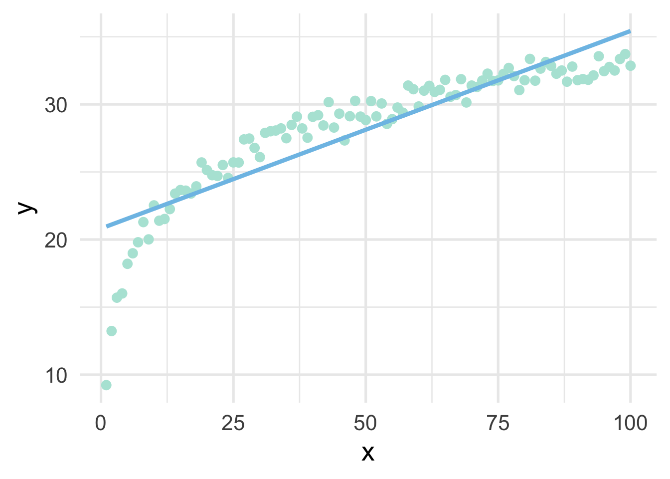
sim <- data.frame(x, y)As you can see from the above, we have simulated the data according to \(\log x\), but our data frame only has \(x\). This is a common situation where we don’t know the true functional form. But of course, if we fit a linear regression model to these data, we’ll end up with high bias, particularly in the lower tail (and issues with heteroscedasticity).
But all we have to do, in this case, is use a log transformation to the \(x\) variable and our linear model fits great.
##   x         y     log_x
## 1 1  9.230453 0.0000000
## 2 2 13.231715 0.6931472
## 3 3 15.700092 1.0986123
## 4 4 16.009766 1.3862944
## 5 5 18.203816 1.6094379
## 6 6 18.982897 1.7917595
sim %>%
mutate(log_x = log(x)) %>%
ggplot(aes(log_x, y)) +
geom_point() +
geom_smooth(method = "lm",
se = FALSE)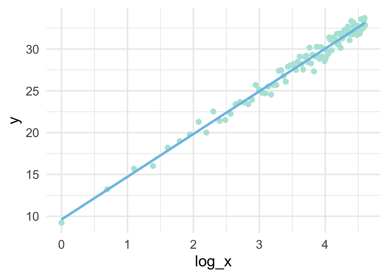
Note that the model is linear in the transformed units, but curvilinear on the raw scale.
sim %>%
  mutate(log_x = log(x)) %>%
  ggplot(aes(x, y)) +
  geom_point() +
  geom_smooth(method = "lm",
              se = FALSE,
              formula = y ~ log(x))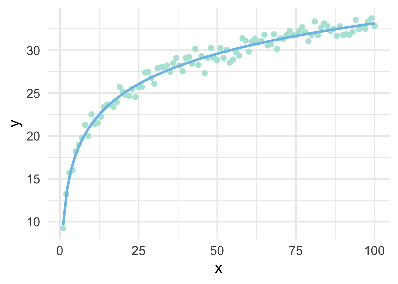
So in this case, a log transformation to the x variable works perfectly (as we would expect, given that we simulated the data to be this way). But how do we know how to transform variables?
31.6.1 Box-Cox and similar transformations
A more general formula for transforming variables is given by the Box-Cox transformation, defined by
\[ \begin{equation} x^* = \begin{cases} \frac{x^\lambda-1}{\lambda}, & \text{if}\ \lambda \neq 0 \\ \log\left(x\right), & \text{if}\ \lambda = 0 \end{cases} \end{equation} \] where \(x\) represents the variable in its raw units, and \(x^*\) represents the transformed variable. The Box-Cox transformation is a power transformation, where the intent is to estimate \(\lambda\). Note that if \(\lambda\) is estimated as zero, the power transformation is the same as a log transformation; otherwise the top portion of the equation is used. Fortunately, specific values of \(\lambda\) map to common transformations.
- \(\lambda = 1\): No transformation
- \(\lambda = 0.5\): square root transformation
- \(\lambda = 0\): log transformation
- \(\lambda = -1\): inverse
Given the above, we would expect that \(\lambda\) would be estimated close to zero with our simulated data. Let’s try using {recipes}. To access the actual \(\lambda\) value, we’ll need to take a brief foray into tidying recipes.
31.6.1.1 Tidying recipes
Let’s first specify the recipe with a Box-Cox transformation to our \(x\) variable.
Now we can tidy the recipe.
## # A tibble: 1 x 6
##   number operation type   trained skip  id
##    <int> <chr>     <chr>  <lgl>   <lgl> <chr>
## 1      1 step      BoxCox FALSE   FALSE BoxCox_dj7Ww
In this case, our recipe is incredibly simple. We have one step, which is a Box-Cox transformation. Let’s make the recipe a bit more complicated just for completeness.
rec <- recipe(y ~ x, data = sim) %>%
  step_impute_linear(all_predictors()) %>%
  step_nzv(all_predictors()) %>%
  step_BoxCox(all_numeric(), -all_outcomes()) %>%
  step_dummy(all_nominal(), -all_outcomes())
Most of these steps won’t do anything in this case, but let’s look at the tidied recipe now.
## # A tibble: 4 x 6
##   number operation type          trained skip  id
##    <int> <chr>     <chr>         <lgl>   <lgl> <chr>
## 1      1 step      impute_linear FALSE   FALSE impute_linear_z6myS
## 2      2 step      nzv           FALSE   FALSE nzv_NxJt6
## 3      3 step      BoxCox        FALSE   FALSE BoxCox_8d2bJ
## 4      4 step      dummy         FALSE   FALSE dummy_J8I0L
Now we have four steps. We can look at any one step by declaring the step number. Let’s look at the linear imputation
## # A tibble: 1 x 3
##   terms            model id
##   <chr>            <lgl> <chr>
## 1 all_predictors() NA    impute_linear_z6myS
Notice there’s nothing there, because at this point the recipe is still just a blueprint. We have to prep() the recipe if we want it to actually do any work. Let’s prep the recipe and try again.
## # A tibble: 1 x 3
##   terms model        id
##   <chr> <named list> <chr>
## 1 x     <lm>         impute_linear_z6myS
And now we can see a linear model has been fit. We can even access the model itself.
## $x
##
## Call:
## NULL
##
## Coefficients:
## (Intercept)
##        50.5
What we get is actually a list of models, one for each predictor. But in this case there’s only one predictor, so the list is only of length 1.
31.6.1.2 Estimating \(\lambda\)
We can do the same thing to find \(\lambda\) by tidying the Box-Cox step
## # A tibble: 1 x 3
##   terms value id
##   <chr> <dbl> <chr>
## 1 x     0.717 BoxCox_8d2bJ
And without any further work we can see that we estimated \(\lambda = 0.72\), which is pretty much directly between a square-root transformation and no transformation. Why did it not estimate a \(log\) transformation as most appropriate? Because the log transformation is only ideal when viewing \(x\) relative to \(y\). Put differently, the Box-Cox transformation is an unsupervised approach that attempts to make each variable approximate a univariate normal distribution. As we’ll see in the next section, there are other methods that can be used to help with issues of non-linearity.
For completeness, let’s see if the transformation helped us. We’ll use \(\lambda = 0.72\) to manually transform \(x\), then plot the result.
# transform x
sim <- sim %>%
  mutate(x_bc = ((x^0.72) - 1) / 0.72)

# fit the model using the transformed data
m <- lm(y ~ x_bc, sim)

# add the model predictions to the data frame
sim <- sim %>%
  mutate(pred = predict(m))

# plot the model fit using raw data on the x-axis
ggplot(sim, aes(x, y)) +
  geom_point() +
  geom_line(aes(y = pred))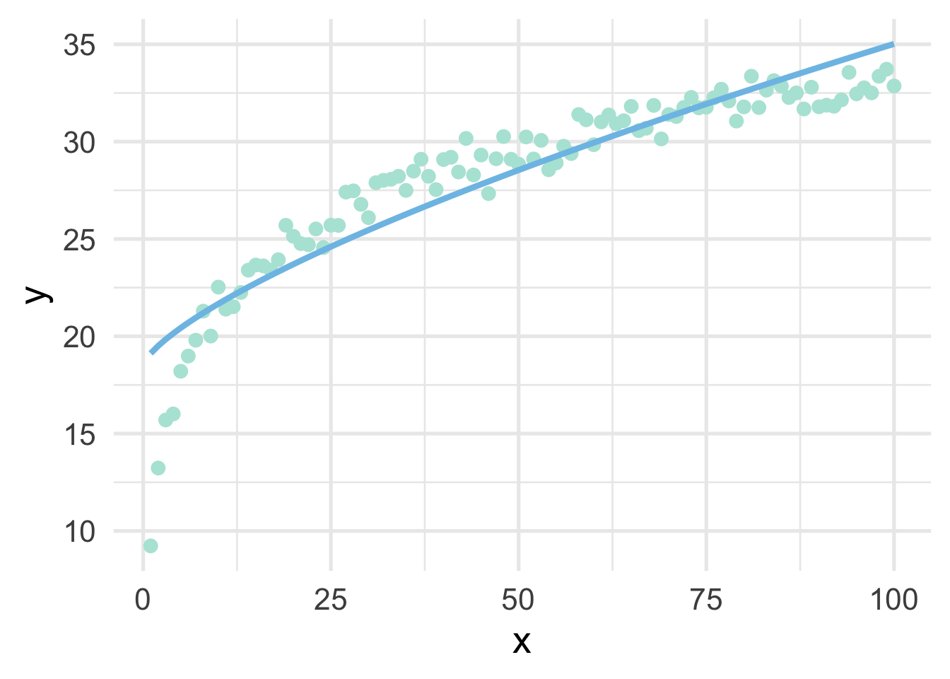
As we can see, it’s better than the raw data, but still insufficient.
31.6.2 An applied example
Let’s look at an applied example. We’ll use the violence data (see the full data dictionary here) and see if we can predict the neighborhoods where the number of murders are greater than zero, using the percentage of people living in poverty and the percentage of people living in dense housing units (more than one person per room) as predictors. Let’s start with a basic plot.
library(sds)
violence <- get_data("violence")

violence <- violence %>%
  mutate(murder = ifelse(murders > 0, "Yes", "No"))

ggplot(violence, aes(pctPoverty, houseVacant)) +
  geom_point(aes(color = murder),
             alpha = 0.5,
             stroke = 0)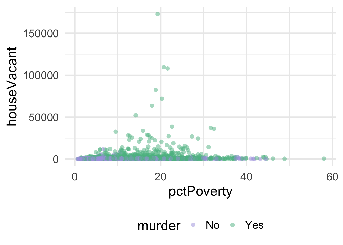
As you can see, it’s pretty difficult to see much separation here. Let’s look at the univariate views of each predictor.
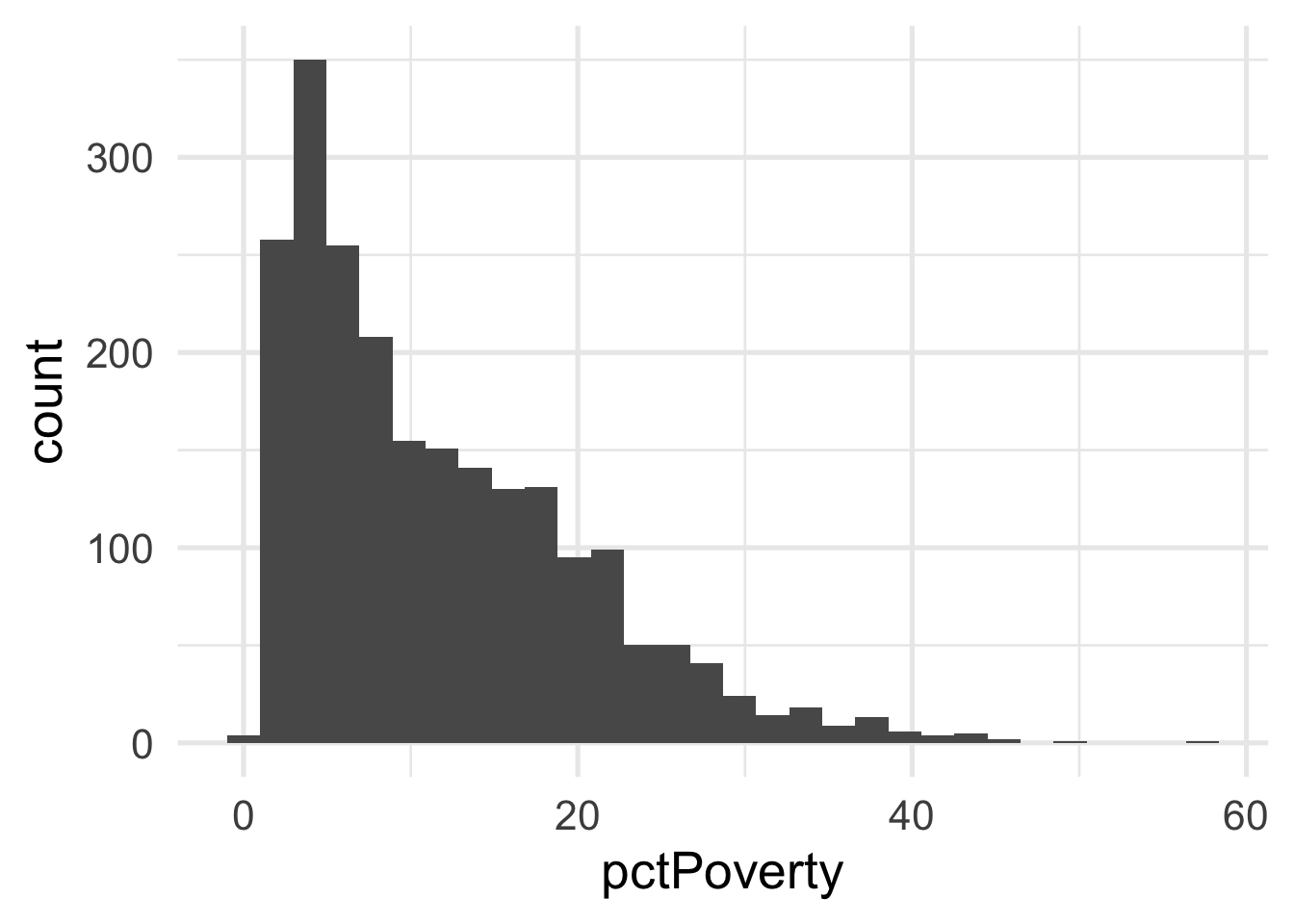
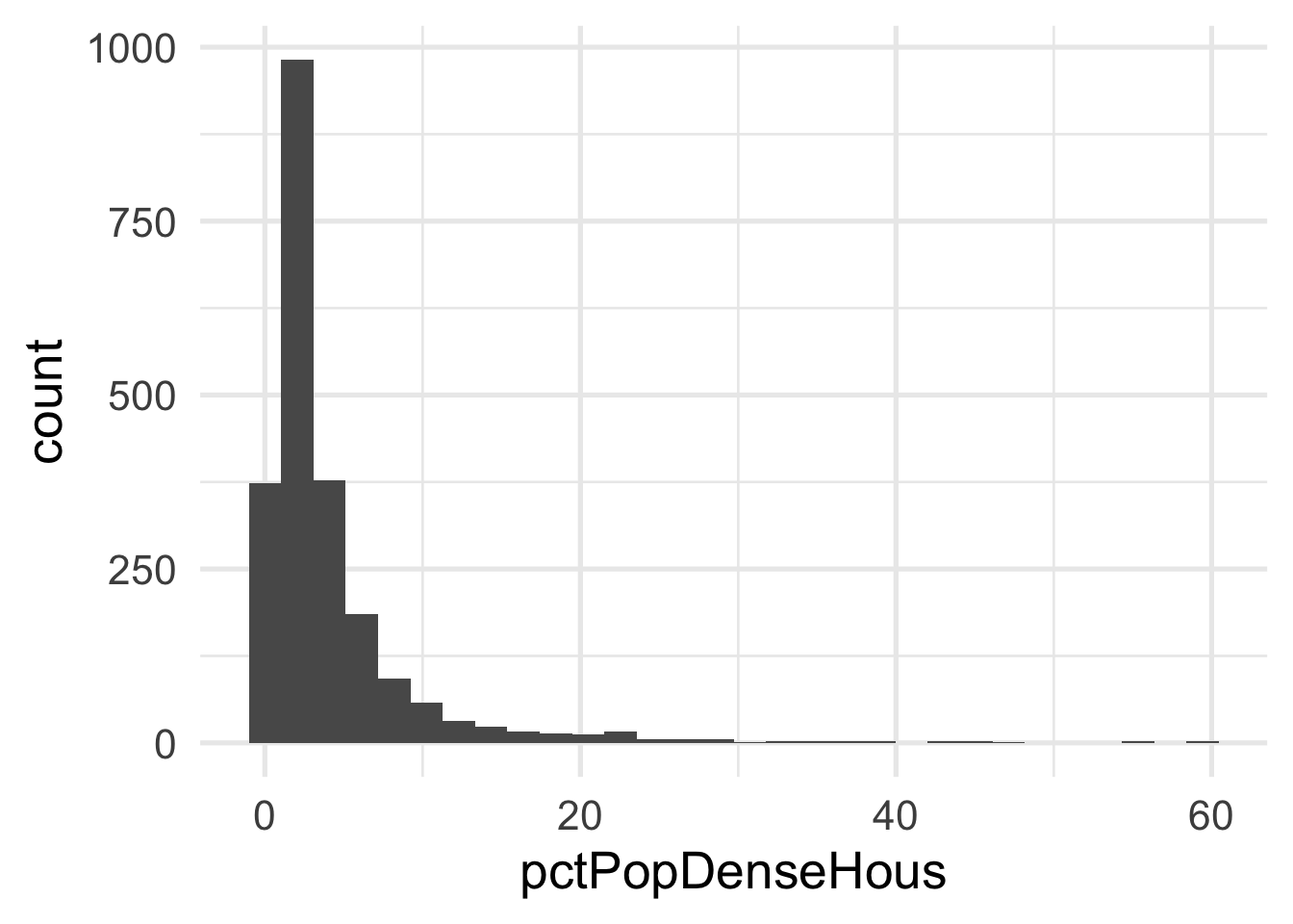
Both predictors are quite skewed. What do they look like after transformation?
murder_rec <- recipe(murder ~ ., violence) %>%
  step_BoxCox(all_numeric(), -all_outcomes())

transformed_murder <- murder_rec %>%
  prep() %>%
  bake(new_data = NULL)

ggplot(transformed_murder, aes(pctPoverty)) +
  geom_histogram()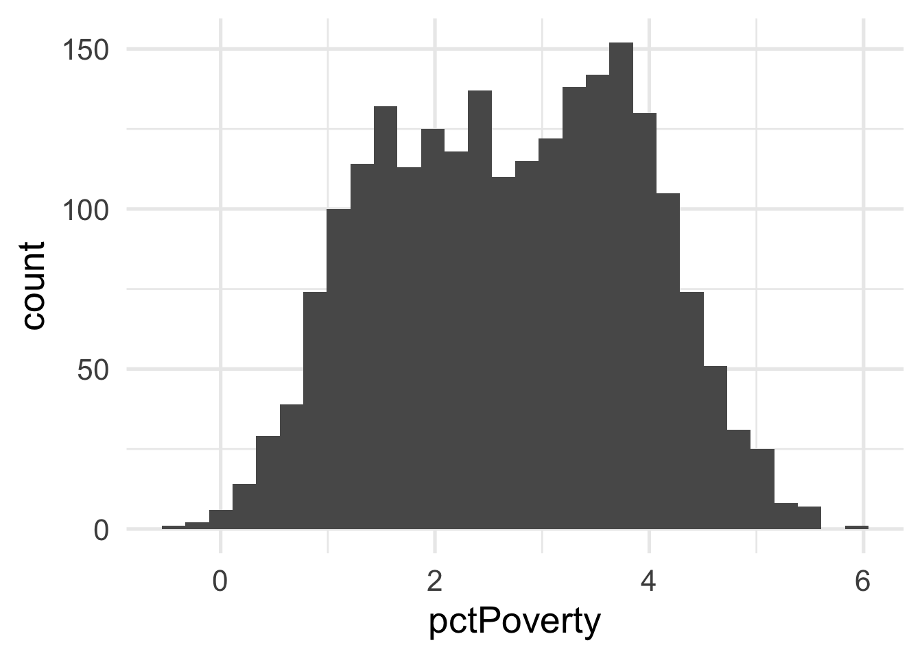
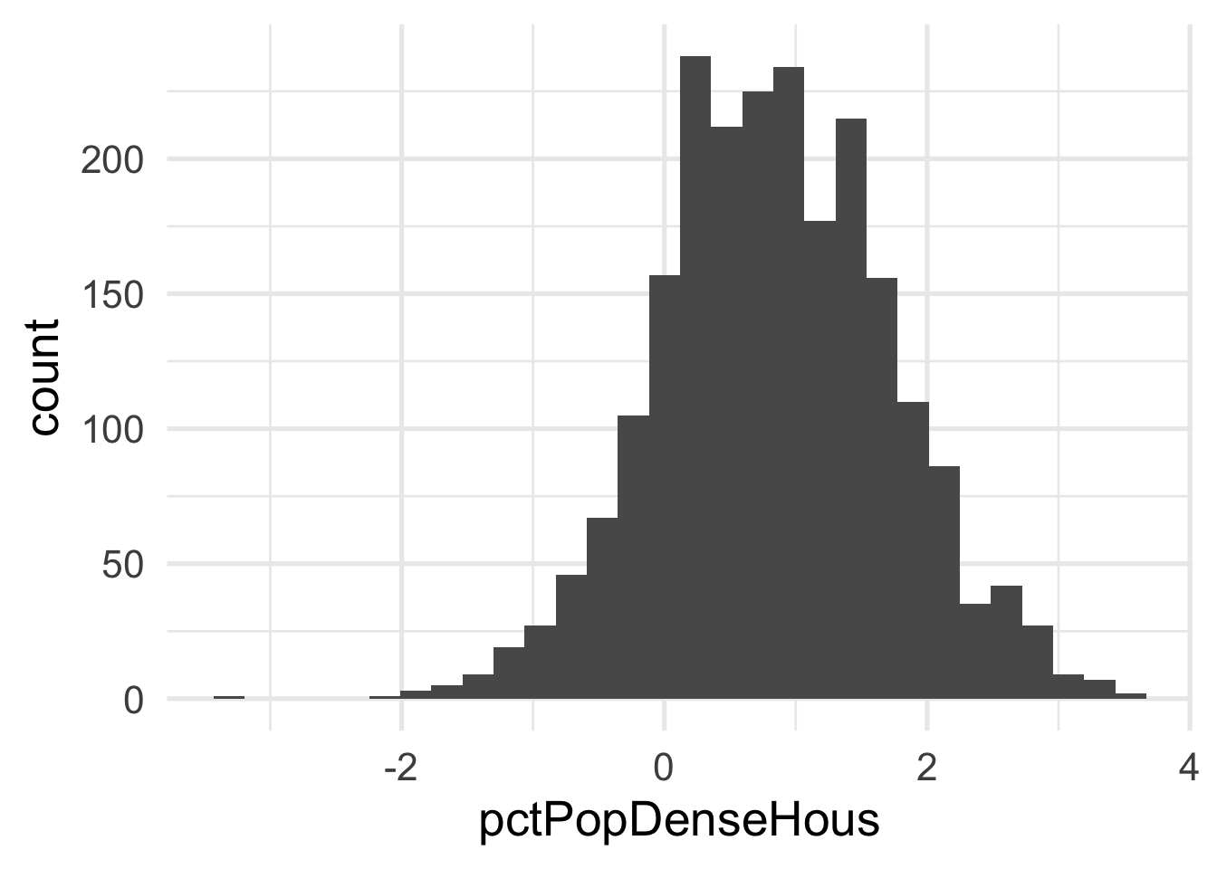
Each of these look considerably better. What about the bivariate view?
ggplot(transformed_murder, aes(pctPoverty, pctPopDenseHous)) +
  geom_point(aes(color = murder),
             alpha = 0.5,
             stroke = 0)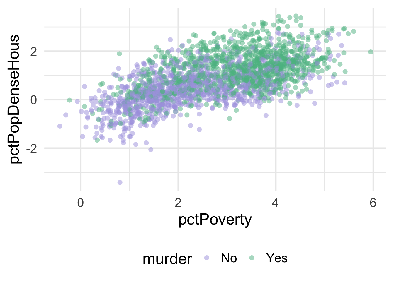
We can much more clearly see the separation here. We could almost draw a diagonal line in the data separating the classes, as below
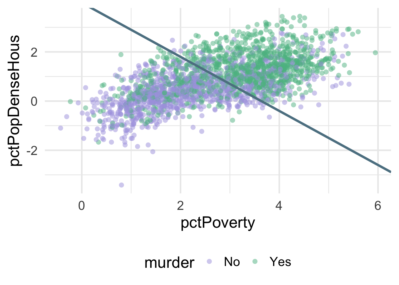
There’s of course still some misclassification going on here, and that line was drawn by just eye-balling it, but even by hand we can do this much easier after the transformation.
What were the lambda values estimated at for these variables? Let’s check.
## # A tibble: 2 x 3
##   terms             value id
##   <chr>             <dbl> <chr>
## 1 pctPoverty       0.177  BoxCox_syfpc
## 2 pctPopDenseHous -0.0856 BoxCox_syfpc
Both are fairly close to zero, implying they are similar to log transformations.
31.7 Nonlinearity
Very regularly, predictor variables will have a nonlinear relation with the outcome. In the previous section, we simulated data to follow a log-linear trend, which is linear on the log scale and curvilinear on the raw scale. As a reminder, the data looked like this
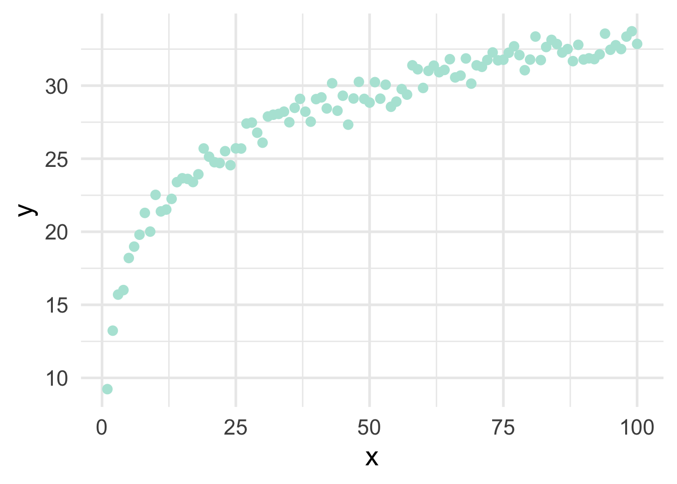
If we just looked at a plot of these data, we’d probably think to ourselves “that looks a whole lot like a log function!”. But let’s pretend for a moment that we’re not quite as brilliant as we actually are and we, say, didn’t plot the data first (always plot the data first!). Or maybe we’re just not all that familiar with the log function, and we didn’t realize that a simple transformation could cure all our woes. How would we go about modeling this? Clearly a linear relation would be insufficient.
There are many different options for modeling curvilinnear relations, but we’ll focus on two: basis expansion via polynomial transformations and natural splines.
Basis expansion is defined, mathematically, as
\[ f(X) = \sum_{m = 1}^M\beta_mh_m(X) \] where \(h_m\) is the \(m\)th transformation of \(X\). Once the transformations are defined, multiple coefficients (\(\beta\)) are estimated to represent each transformation, which sum to form the non-linear trend. However, the model is itself still linear. We illustrate below.
31.7.1 Polynomial transformations
Polynomial transformations include the variable in its raw units, plus additional (basis expansion) units raised to a given power. For example, a cubic trend could be fit by transforming \(X\) into \(X\), \(X^2\), and \(X^3\), and estimating coefficients for each. Let’s do this manually with the sim data from above.
# remove variables from previous example
# keep only `x` and `y`
sim <- sim %>%
select(x, y)
sim <- sim %>%
mutate(x2 = x^2,
x3 = x^3) %>%
select(starts_with("x"), y)
head(sim)## x x2 x3 y
## 1 1 1 1 9.230453
## 2 2 4 8 13.231715
## 3 3 9 27 15.700092
## 4 4 16 64 16.009766
## 5 5 25 125 18.203816
## 6 6 36 216 18.982897Now let’s fit a model to the data using the polynomial expansion, and plot the result.
## x x2 x3 y poly_pred
## 1 1 1 1 9.230453 14.99051
## 2 2 4 8 13.231715 15.63371
## 3 3 9 27 15.700092 16.25849
## 4 4 16 64 16.009766 16.86514
## 5 5 25 125 18.203816 17.45393
## 6 6 36 216 18.982897 18.02516
Not bad!
Now let’s replicate it using {recipes}.
sim <- sim %>%
select(x, y)
poly_rec <- recipe(y ~ ., sim) %>%
step_poly(all_predictors(), degree = 3)
poly_d <- poly_rec %>%
prep() %>%
bake(new_data = NULL)
poly_d## # A tibble: 100 x 4
## y x_poly_1 x_poly_2 x_poly_3
## <dbl> <dbl> <dbl> <dbl>
## 1 9.23 -0.171 0.217 -0.249
## 2 13.2 -0.168 0.204 -0.219
## 3 15.7 -0.165 0.191 -0.190
## 4 16.0 -0.161 0.178 -0.163
## 5 18.2 -0.158 0.166 -0.137
## 6 19.0 -0.154 0.154 -0.113
## 7 19.8 -0.151 0.142 -0.0904
## 8 21.3 -0.147 0.131 -0.0690
## 9 20.0 -0.144 0.119 -0.0489
## 10 22.5 -0.140 0.108 -0.0302
## # … with 90 more rowsNotice that these values look quite a bit different than the ones we had before because these are orthogonal polynomials. Orthogonal polynomials have some advantages over raw polynomials, including that, in a standard linear regression modeling framework, each higher-order term can be directly evaluated for its contribution to the model. This is mostly because non-orthogonal polynomials are highly correlated. However, the fitted values remain the same, as we can see below.
poly_m2 <- lm(y ~ ., data = poly_d)
sim <- sim %>%
mutate(poly_pred2 = predict(poly_m2))
ggplot(sim, aes(x, y)) +
geom_point() +
geom_line(aes(y = poly_pred2))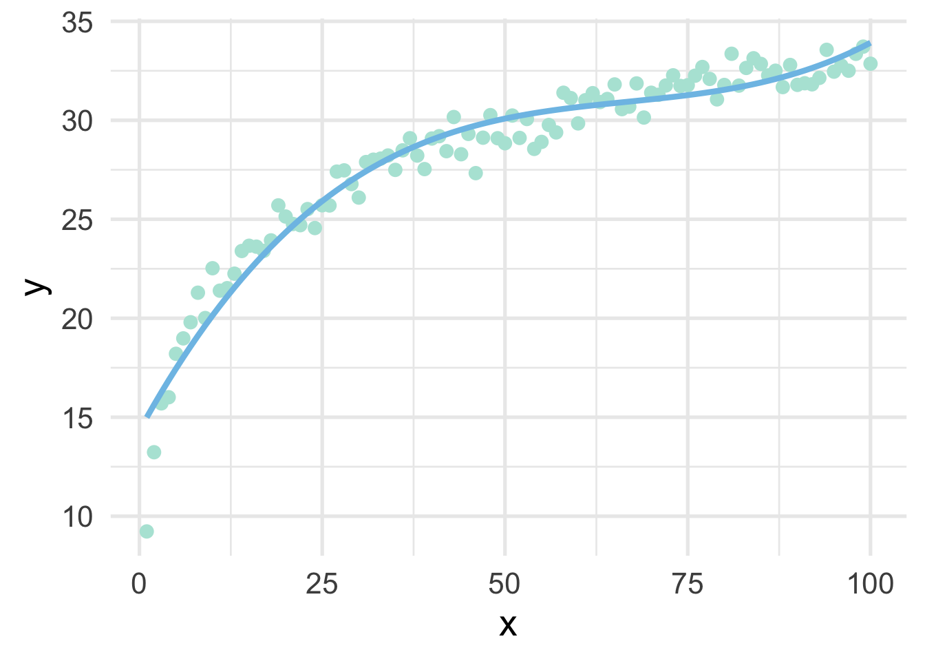
But let’s be even more precise and verify that they are, indeed, identical in their fitted values.
## [1] TRUEThis shows that, to seven decimal places, the results are identical (note, the only reason I had to round at all was because of floating point hell).
31.7.2 Splines
When thinking about splines, we find it most helpful to first think about discontinuous splines. Splines divide up the “x” region of the predictor into bins, and fits a model within each bin. Let’s first look at a very simple model, where we divide our sim dataset into lower and upper portions.
# get only x and y back
sim <- sim %>%
  select(x, y)

# Fit a model to the lower and upper parts
lower_part <- lm(y ~ x, filter(sim, x <= 50))
upper_part <- lm(y ~ x, filter(sim, x > 50))

# make predictions from each part
lower_pred <- predict(lower_part, newdata = data.frame(x = 0:50))
upper_pred <- predict(upper_part, newdata = data.frame(x = 51:100))

# graph the results
ggplot(sim, aes(x, y)) +
  annotate("rect",
           xmin = -Inf, ymin = -Inf, ymax = Inf, xmax = 50,
           fill = "#7EC1E7", alpha = 0.3) +
  geom_point() +
  geom_line(data = data.frame(x = 0:50, y = lower_pred)) +
  geom_line(data = data.frame(x = 51:100, y = upper_pred))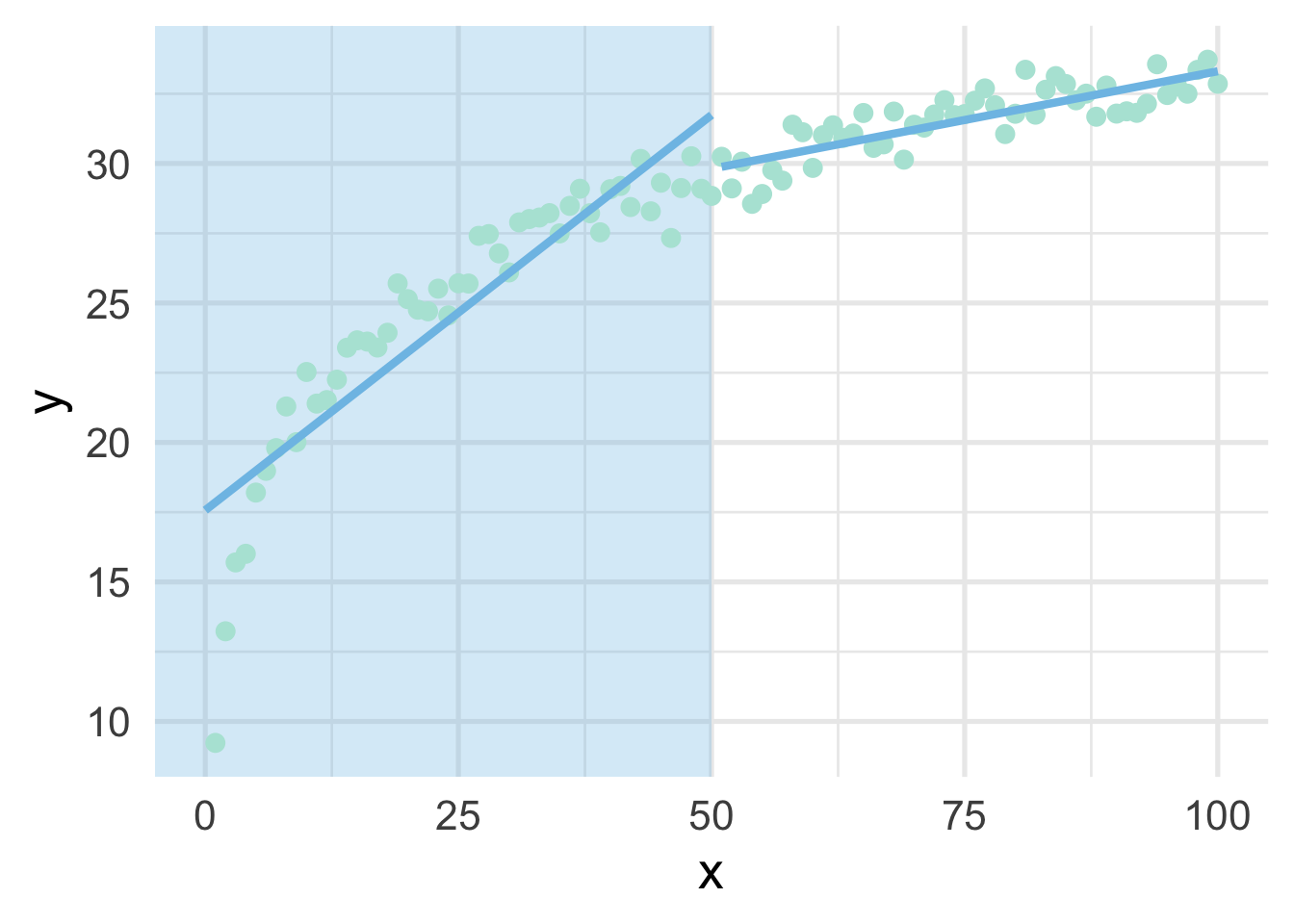
As you can see, this gets at the same non-linearity, but with two models. We can better approximate the curve by increasings the number of “bins” in the x-axis. Let’s use 10 bins instead.
ten_bins <- sim %>%
  mutate(tens = as.integer(x/10)) %>%
  group_by(tens) %>%
  nest() %>%
  mutate(m = map(data, ~lm(y ~ x, .x)),
         pred_frame = map2(data, m, ~data.frame(x = .x$x, y = predict(.y))))

ggplot(sim, aes(x, y)) +
  geom_vline(xintercept = seq(10, 90, 10),
             color = "gray30") +
  geom_point() +
  map(ten_bins$pred_frame, ~geom_line(data = .x))
This approximates the underlying curve quite well.
We can try again by fitting polynomial models within each bin to see if that helps. Note we’ve place the point where x == 100 into the bin for 9, because there’s only one point in that bin and the model can’t be fit to a single point.
ten_bins <- sim %>%
  mutate(tens = as.integer(x / 10),
         tens = ifelse(tens == 10, 9, tens)) %>%
  group_by(tens) %>%
  nest() %>%
  mutate(m = map(data, ~lm(y ~ poly(x, 3), .x)),
         pred_frame = map2(data, m, ~data.frame(x = .x$x,
                                                y = predict(.y))))

ggplot(sim, aes(x, y)) +
  geom_vline(xintercept = seq(10, 90, 10),
             color = "#7EC1E7") +
  geom_point() +
  map(ten_bins$pred_frame, ~geom_line(data = .x))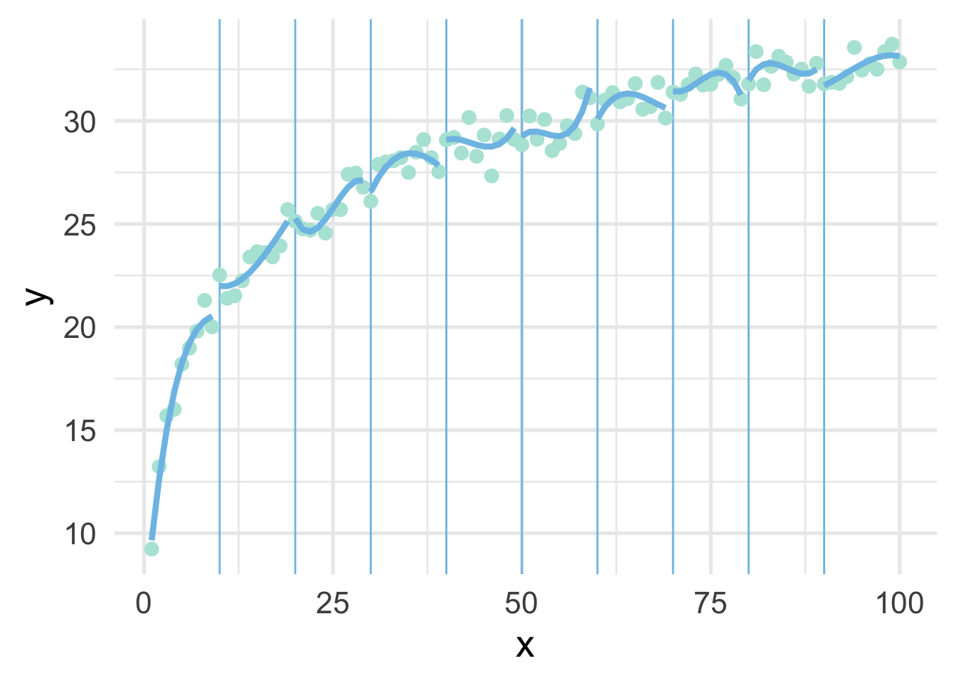
But now we have 10 different models! Wouldn’t it be better if we had a single curve? YES! Of course. And that’s exactly what a spline is. It forces each of these curves to connect in a smooth way. The points defining the bins are referred to as “knots”.
Let’s fit a spline to these data, using 8 “interior” knots (for 10 knots total, including one on each boundary).
library(splines)
ns_mod <- lm(y ~ ns(x, 8), sim)

ggplot(sim, aes(x, y)) +
  geom_point() +
  geom_line(data = data.frame(x = 1:100, y = predict(ns_mod)))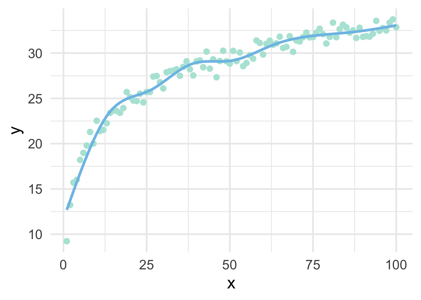
And now we have our single curve! The purpose of our discussion here is to build conceptual understandings of splines, and we will therefore not go into the mathematics behind the constraints leading to a single curve. However, for those interested, we recommend Hastie, Tibshirani, and Friedman.
One of the drawbacks of polynomial regression is that they can be wild in the tails. Natural splines avoid this problem by constraining the tails of the curve to be linear. Sometimes, however, this property may not be desirable, and that’s when we instead use a B-spline.
bs_mod <- lm(y ~ bs(x, 8), sim)

ggplot(sim, aes(x, y)) +
  geom_point() +
  geom_line(data = data.frame(x = 1:100, y = predict(bs_mod)))
Let’s look at the true data-generating curve with each of the splines, omitting the points for clarity.
ns_d <- data.frame(x = 1:100,
                   y = predict(ns_mod),
                   method = "Natural Spline")
bs_d <- data.frame(x = 1:100,
                   y = predict(bs_mod),
                   method = "B-Spline")

ggplot(rbind(ns_d, bs_d), aes(x, y)) +
  geom_smooth(data = sim,
              method = "lm",
              formula = y ~ log(x),
              se = FALSE,
              color = "#5E8192") +
  geom_line(aes(color = method)) +
  facet_wrap(~method)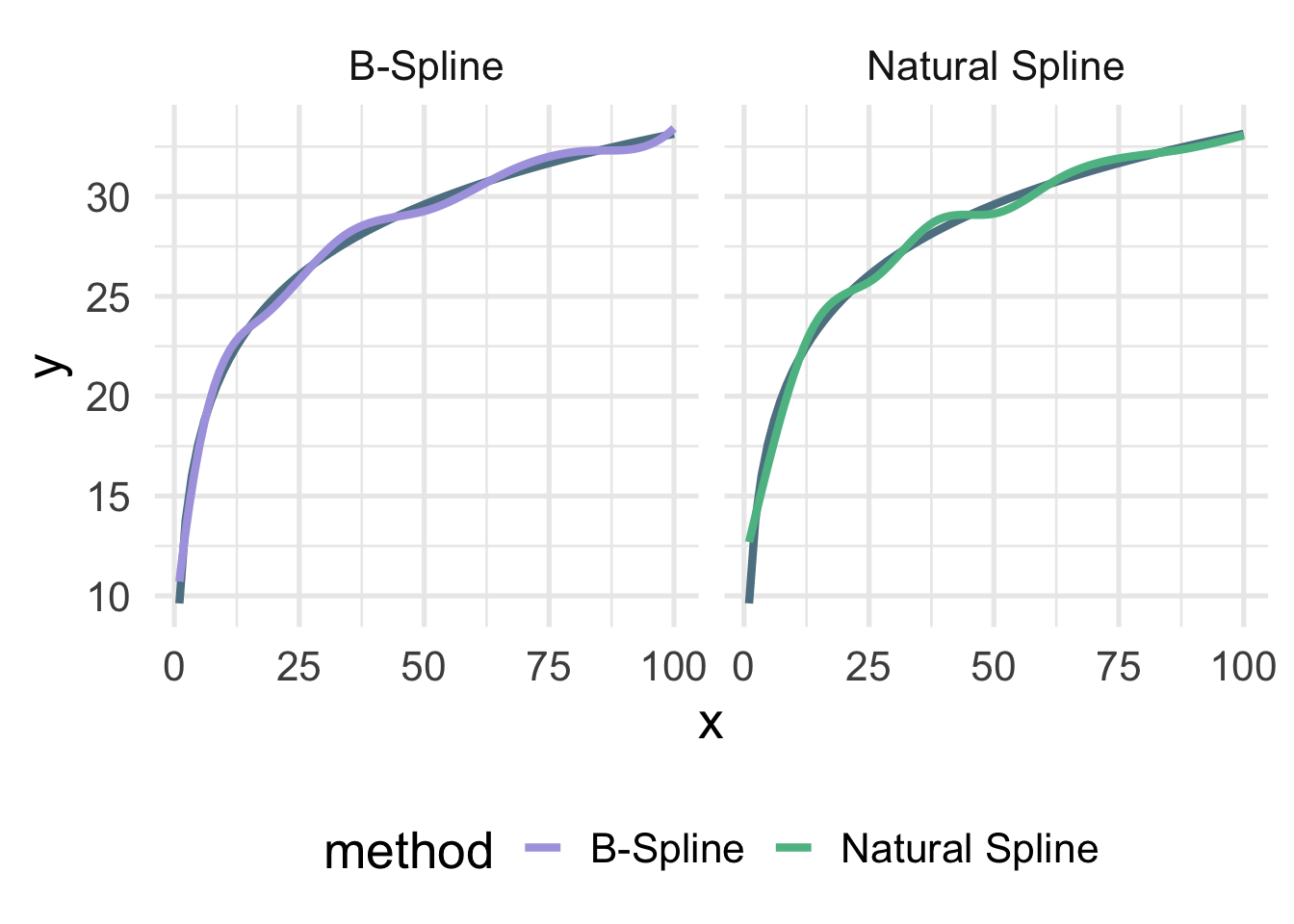
Both are quite close, but you can see the natural spline does not dip quite as close to the true value for zero as the B-spline. It’s also a tiny bit more wiggly in the upper tail (because it’s not constrained to be linear). The number of knots is also likely a bit too high here and was chosen fairly randomly.
31.7.2.1 Basis expansion with {recipes}
Basis expansion via recipes proceeds in much the same way as we’ve seen before. We just specify a step identifying the the type of basis expansion we want to conduct, along with any additional arguments like the degrees of freedom (number of knots).
Let’s try building a dataset using basis expansion with a B-Spline
bs_d <- recipe(y ~ x, data = sim) %>%
  step_bs(x, deg_free = 8) %>%
  prep() %>%
  bake(new_data = NULL)

bs_d
## # A tibble: 100 x 9
## y x_bs_1 x_bs_2 x_bs_3 x_bs_4 x_bs_5 x_bs_6 x_bs_7 x_bs_8
## <dbl> <dbl> <dbl> <dbl> <dbl> <dbl> <dbl> <dbl> <dbl>
## 1 9.23 0 0 0 0 0 0 0 0
## 2 13.2 0.166 0.00531 0.0000371 0 0 0 0 0
## 3 15.7 0.301 0.0204 0.000297 0 0 0 0 0
## 4 16.0 0.407 0.0441 0.00100 0 0 0 0 0
## 5 18.2 0.488 0.0751 0.00237 0 0 0 0 0
## 6 19.0 0.545 0.112 0.00464 0 0 0 0 0
## 7 19.8 0.580 0.154 0.00801 0 0 0 0 0
## 8 21.3 0.596 0.200 0.0127 0 0 0 0 0
## 9 20.0 0.596 0.248 0.0190 0 0 0 0 0
## 10 22.5 0.582 0.298 0.0270 0 0 0 0 0
## # … with 90 more rowsAnd as you can see, we get similar output to polynomial regression, but we’re just using a spline for our basis expansion now instead of polynomials. Note that the degrees of freedom can also be set to tune() and trained withing tune::tune_grid(). In other words, the amount of basis expansion (degree of “wiggliness”) can be treated as a hyperparamter to be tuned.
Once the basis expansion is conducted, we can model it just like any other linear model.
bs_mod_2 <- lm(y ~ x_bs_1 + x_bs_2 + x_bs_3 +
                     x_bs_4 + x_bs_5 + x_bs_6 +
                     x_bs_7 + x_bs_8,
                 data = bs_d)
And this will give us the same results we got before.
## [1] TRUETo use polynomial transformations or natural splines instead, we would just use step_poly() or step_ns(), respectively.
One rather important note on tuning splines, you will probably want to avoid using code like
## Data Recipe
##
## Inputs:
##
##       role #variables
##    outcome          1
##  predictor        147
##
## Operations:
##
## Natural Splines on all_predictors()
because this will constrain the smooth to be the same for all predictors. Instead, use exploratory analyses and plots to figure out which variables should be fit with splines, and then tune them separately. For example
recipe(murders ~ ., data = violence) %>%
  step_ns(pctPoverty, deg_free = tune()) %>%
  step_ns(houseVacant, deg_free = tune())
## Data Recipe
##
## Inputs:
##
## role #variables
## outcome 1
## predictor 147
##
## Operations:
##
## Natural Splines on pctPoverty
## Natural Splines on houseVacantOf course, the more splines you are tuning, the more computationally expensive it will become, so you’ll need to balance this with your expected return in model improvement (i.e., you likely can’t tune every predictor in your dataset).
31.8 Interactions
An interaction occurs when the slope, or relation, between one variable and the outcome depends upon a second variable. This is also often referred to as moderation or a moderating variable. For example, consider data that look like this:
benchmarks <- get_data("benchmarks")

ggplot(benchmarks, aes(rdg_fall, rdg_spr)) +
  geom_point(color = "gray70") +
  geom_smooth(aes(color = ell),
                  method = "lm")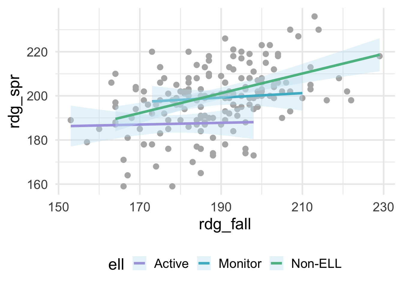
where ell stands for “English language learner”. The plot above shows the relation between students scores on a reading assessment administered in the fall and the spring by ell status. Notice that the slope for Non-ELL is markedly steeper than the other two groups. ell status thus moderates the relation between the fall and spring assessment scores. If we’re fitting a model within a linear regression framework, we’ll want to make sure that we model the slopes separately for each of these groups. Otherwise, we would be leaving out important structure in the data, and our model performance would suffer. Interactions are powerful and important to consider, particularly if there is strong theory (or empirical evidence) suggesting that an interaction exists. However, they are not needed in many frameworks and can be derived from the data directly (e.g., tree-based methods, where the degree of possible interaction is determined by the depth of the tree). In this section, we therefore focus on interactions within a linear regression framework.
31.8.1 Creating interactions “by hand”
Even with base R, modeling interactions is pretty straightforward. In the above, we would just specify something like
or equivalently,
However, this is doing some work under the hood for you which might go unnoticed. First, it’s dummy-coding ell, then it’s creating, in this case, two new variables that are equal to \(ELL_{Monitor} \times Rdg_{fall}\) and \(ELL_{Non-ELL} \times Rdg_{fall}\) (with \(ELL_{Active}\) set as the reference group by default).
Let’s try doing this manually. First we need to dummy code ell. To make things a bit more clear, I’ll only select the variables here that we’re using in our modeling.
dummies <- benchmarks %>%
  select(rdg_fall, ell, rdg_spr) %>%
  mutate(ell_monitor = ifelse(ell == "Monitor", 1, 0),
         ell_non = ifelse(ell == "Non-ELL", 1, 0),)
dummies
## # A tibble: 174 x 5
## rdg_fall ell rdg_spr ell_monitor ell_non
## <dbl> <chr> <dbl> <dbl> <dbl>
## 1 181 Active 194 0 0
## 2 166 Non-ELL 159 0 1
## 3 216 Non-ELL 198 0 1
## 4 203 Non-ELL 204 0 1
## 5 198 Active 173 0 0
## 6 188 Active 173 0 0
## 7 202 Monitor 200 1 0
## 8 182 Active 206 0 0
## 9 194 Non-ELL 191 0 1
## 10 170 Active 185 0 0
## # … with 164 more rowsNext, we’ll multiply each of these dummy variables by rdg_fall.
interactions <- dummies %>%
  mutate(fall_monitor = rdg_fall * ell_monitor,
         fall_non = rdg_fall * ell_non)
interactions
## # A tibble: 174 x 7
## rdg_fall ell rdg_spr ell_monitor ell_non fall_monitor fall_non
## <dbl> <chr> <dbl> <dbl> <dbl> <dbl> <dbl>
## 1 181 Active 194 0 0 0 0
## 2 166 Non-ELL 159 0 1 0 166
## 3 216 Non-ELL 198 0 1 0 216
## 4 203 Non-ELL 204 0 1 0 203
## 5 198 Active 173 0 0 0 0
## 6 188 Active 173 0 0 0 0
## 7 202 Monitor 200 1 0 202 0
## 8 182 Active 206 0 0 0 0
## 9 194 Non-ELL 191 0 1 0 194
## 10 170 Active 185 0 0 0 0
## # … with 164 more rowsAs would be expected, these values are zero if they are not for the corresponding group, and are otherwise equal to rdg_fall. If we enter all these variables in our model, then our model intercept will represent the intercept for the active group, with the corresponding slope estimated by rdg_fall. The ell_monitor and ell_non terms represent the intercepts for the monitor and non-ELL groups, respectively, and each of these slopes are estimated by the corresponding interaction. Let’s try.
m_byhand <- lm(rdg_spr ~ rdg_fall + ell_monitor + ell_non +
                         fall_monitor + fall_non,
               data = interactions)
summary(m_byhand)
##
## Call:
## lm(formula = rdg_spr ~ rdg_fall + ell_monitor + ell_non + fall_monitor +
## fall_non, data = interactions)
##
## Residuals:
## Min 1Q Median 3Q Max
## -36.812 -7.307 -0.100 8.616 26.693
##
## Coefficients:
## Estimate Std. Error t value Pr(>|t|)
## (Intercept) 180.29666 32.95228 5.471 1.6e-07 ***
## rdg_fall 0.03939 0.18459 0.213 0.8313
## ell_monitor -0.47286 53.18886 -0.009 0.9929
## ell_non -64.12123 36.80395 -1.742 0.0833 .
## fall_monitor 0.06262 0.28669 0.218 0.8274
## fall_non 0.40801 0.20346 2.005 0.0465 *
## ---
## Signif. codes: 0 '***' 0.001 '**' 0.01 '*' 0.05 '.' 0.1 ' ' 1
##
## Residual standard error: 12.37 on 168 degrees of freedom
## Multiple R-squared: 0.2652, Adjusted R-squared: 0.2433
## F-statistic: 12.13 on 5 and 168 DF, p-value: 4.874e-10And we can verify that this does, indeed, get us the same results that we would have obtained with the shortcut syntax with base R.
##
## Call:
## lm(formula = rdg_spr ~ rdg_fall * ell, data = benchmarks)
##
## Residuals:
##     Min      1Q  Median      3Q     Max
## -36.812  -7.307  -0.100   8.616  26.693
##
## Coefficients:
##                      Estimate Std. Error t value Pr(>|t|)
## (Intercept)         180.29666   32.95228   5.471  1.6e-07 ***
## rdg_fall              0.03939    0.18459   0.213   0.8313
## ellMonitor           -0.47286   53.18886  -0.009   0.9929
## ellNon-ELL          -64.12123   36.80395  -1.742   0.0833 .
## rdg_fall:ellMonitor   0.06262    0.28669   0.218   0.8274
## rdg_fall:ellNon-ELL   0.40801    0.20346   2.005   0.0465 *
## ---
## Signif. codes:  0 '***' 0.001 '**' 0.01 '*' 0.05 '.' 0.1 ' ' 1
##
## Residual standard error: 12.37 on 168 degrees of freedom
## Multiple R-squared:  0.2652, Adjusted R-squared:  0.2433
## F-statistic: 12.13 on 5 and 168 DF,  p-value: 4.874e-10
31.8.2 Creating interactions with {recipes}
Specifying interactions in a recipe is similar to other steps, with one small exception, which is that the use of the tilde, ~, is required. Note that, once again, order does matter, and you should always do your dummy coding before specifying interactions with categorical variables. In the example before, this would correspond to:
recipe(rdg_spr ~ rdg_fall + ell, benchmarks) %>%
  step_dummy(all_nominal()) %>%
  step_interact(~rdg_fall:starts_with("ell")) %>%
  prep() %>%
  bake(new_data = NULL)
## # A tibble: 174 x 6
## rdg_fall rdg_spr ell_Monitor ell_Non.ELL rdg_fall_x_ell_Mo… rdg_fall_x_ell_N…
## <dbl> <dbl> <dbl> <dbl> <dbl> <dbl>
## 1 181 194 0 0 0 0
## 2 166 159 0 1 0 166
## 3 216 198 0 1 0 216
## 4 203 204 0 1 0 203
## 5 198 173 0 0 0 0
## 6 188 173 0 0 0 0
## 7 202 200 1 0 202 0
## 8 182 206 0 0 0 0
## 9 194 191 0 1 0 194
## 10 170 185 0 0 0 0
## # … with 164 more rowsThere are a few things to mention here. First, the data look identical (minus the column names) to what we created by hand, so that’s good news. However, we also used starts_with() here, rather than just specifying something like step_interact(~rdg_fall:ell). This is because after dummy coding, the column names change (as you can see in the above). By specifying starts_with(), we are ensuring that we get all the interactions we need. If we forget this step, we end up with the wrong output, along with a warning.
recipe(rdg_spr ~ rdg_fall + ell, benchmarks) %>%
  step_dummy(all_nominal()) %>%
  step_interact(~rdg_fall:ell) %>%
  prep() %>%
  bake(new_data = NULL)
## Warning: Interaction specification failed for: ~rdg_fall:ell. No interactions
## will be created.## # A tibble: 174 x 4
## rdg_fall rdg_spr ell_Monitor ell_Non.ELL
## <dbl> <dbl> <dbl> <dbl>
## 1 181 194 0 0
## 2 166 159 0 1
## 3 216 198 0 1
## 4 203 204 0 1
## 5 198 173 0 0
## 6 188 173 0 0
## 7 202 200 1 0
## 8 182 206 0 0
## 9 194 191 0 1
## 10 170 185 0 0
## # … with 164 more rowsThis warning occurs because R is trying to find a column called ell to multiply with rdg_fall, but no such variable exists after dummy coding.
31.9 PCA
For some sets of models (such as linear regression), highly correlated variables may cause model instability or, perhaps more importantly, lead to wider confidence intervals around model predictions (i.e., how confident we are about our prediction). In these cases, it may help to collapse these variables, while still accounting for the majority of the variance. This is the basic idea behind Principal Components Analysis (PCA). You use PCA to collapse sets of variables into principal components, reducing the dimensionality of your data while maintaining \(X\) percent of the original variation in the data. Reducing the dimensionality generally has an associated cost of higher model bias. However, it will also nearly always reduce model variability. The proportion of the original variability to maintain can thus be considered a tuning parameter, balancing bias with variance.
Probably my favorite discussion of PCA comes from a discussion on CrossValidated on how to make sense of PCA. The opening poster asked how you would explain PCA to a layman and why it’s needed. The entire thread is worth reading through, and there’s a particularly nice example from JD Long comparing the first principal component to the line of best fit in linear regression.
For our purposes, we’re primarily interested in what proportion of the total variability in the independent variables we should maintain. That is, can we improve our model performance by collapsing groups of (correlated) columns into a smaller set of principal components?
31.9.1 PCA with {recipes}
Let’s move back to our full dataset. Our final recipe looked like this.
rec <- recipe(score ~ ., train) %>%
  update_role(contains("id"), ncessch, new_role = "id vars") %>%
  step_mutate(lang_cd = factor(ifelse(is.na(lang_cd), "E", lang_cd)),
              tst_dt = lubridate::mdy_hms(tst_dt)) %>%
  step_zv(all_predictors()) %>%
  step_dummy(all_nominal())
To conduct PCA we need to make sure that
- All variables are numeric
- All variables are on the same scale
- There is no missing data
Our recipe above ensures all variables are numeric, but it doesn’t handle missing data, and there is no standardization of variables. Let’s update this recipe to make sure it’s ready for PCA.
rec <- recipe(score ~ ., train) %>%
  step_mutate(tst_dt = lubridate::mdy_hms(tst_dt)) %>%
  update_role(contains("id"), ncessch, new_role = "id vars") %>%
  step_zv(all_predictors()) %>%
  step_unknown(all_nominal()) %>%
  step_medianimpute(all_numeric(), -all_outcomes(), -has_role("id vars")) %>%
  step_normalize(all_numeric(), -all_outcomes(), -has_role("id vars")) %>%
  step_dummy(all_nominal(), -has_role("id vars"))
The above is not a whole lot more complex than our original recipe. It just assigns an "unknown" level to the nominal variables and imputes the remaining numeric variables with the median of that variable. It then normalizes all variables and dummy codes the nominal variables.
This recipe gives us a data frame with many columns. Specifically:
## [1] 80Let’s create a recipe that retains 80% of the total variability with a smaller set of principal components.
Notice that we just have to specify the threshold of variance we want to maintain. How many columns do we have now?
## [1] 10We’ve dramatically reduced the dimensionality in the data, while still retaining 80% of the total variability.
An alternative method is to specify the number of components we want. For example, let’s extract only the first five components.
I generally prefer the former because, if we’re thinking about PCA through a predictive modeling framework, we’re probably less concerned with the number of components and more concerned with the variation they represent.
So how do we know how much of the variabilty we should retain? This is a difficult question, but sometimes plots of the principal components can help. Let’s look at the five components we just extracted. If we prep the recipe, you’ll see there’s some extra information we can access.
## [1] "var_info"       "term_info"      "steps"          "template"
## [5] "retained"       "tr_info"        "orig_lvls"      "last_term_info"
If we access the steps we can get additional information. The PCA step is the seventh, and it has the following elements stored in the list.
##  [1] "terms"     "role"      "trained"   "num_comp"  "threshold" "options"
##  [7] "res"       "prefix"    "skip"      "id"
Let’s look into res.
## [1] "sdev" "rotation" "center" "scale"And now we get what we’ve been (perhaps unknowingly to you, dear reader) looking for, the sdev object, which lists the standard deviation of each principal component. We can look at how much variance each component accounts for, as follows:
##  [1] 7.503092e-01 5.138784e-02 5.055445e-02 4.135567e-02 2.388100e-02
##  [6] 1.154347e-02 8.222078e-03 8.051600e-03 7.564274e-03 7.346244e-03
## [11] 5.926695e-03 5.187219e-03 4.420626e-03 3.803443e-03 3.418581e-03
## [16] 2.536214e-03 2.344631e-03 1.533003e-03 1.516079e-03 1.397730e-03
## [21] 1.170231e-03 1.071354e-03 1.001754e-03 8.622161e-04 7.596821e-04
## [26] 7.042076e-04 4.803264e-04 3.837786e-04 3.359652e-04 3.219790e-04
## [31] 1.786945e-04 1.426193e-04 7.831676e-05 6.866070e-05 3.886009e-05
## [36] 3.175614e-05 2.647517e-05 2.034393e-05 1.580665e-05 6.911480e-06
## [41] 1.361666e-30 5.047925e-31 1.214792e-32 9.199957e-33 6.414887e-33
## [46] 6.414887e-33 6.414887e-33 6.414887e-33 6.414887e-33 6.414887e-33
## [51] 6.414887e-33 6.414887e-33 6.414887e-33 6.414887e-33 6.414887e-33
## [56] 6.414887e-33 6.414887e-33 6.414887e-33 6.414887e-33 6.414887e-33
## [61] 6.414887e-33 6.414887e-33 6.414887e-33 6.414887e-33 6.414887e-33
## [66] 6.414887e-33 6.414887e-33 6.414887e-33 6.414887e-33 6.414887e-33
## [71] 6.414887e-33 6.414887e-33
That’s difficult to read. Let’s plot it instead
pcs <- data.frame(pc = paste0("PC", 1:length(pvar)),
                  percent_var = pvar) %>%
  mutate(pc = reorder(factor(pc), percent_var))

ggplot(pcs, aes(pc, percent_var)) +
  geom_col() +
  coord_flip() +
  scale_y_continuous(expand = c(0, 0)) # move this to a book theme for plots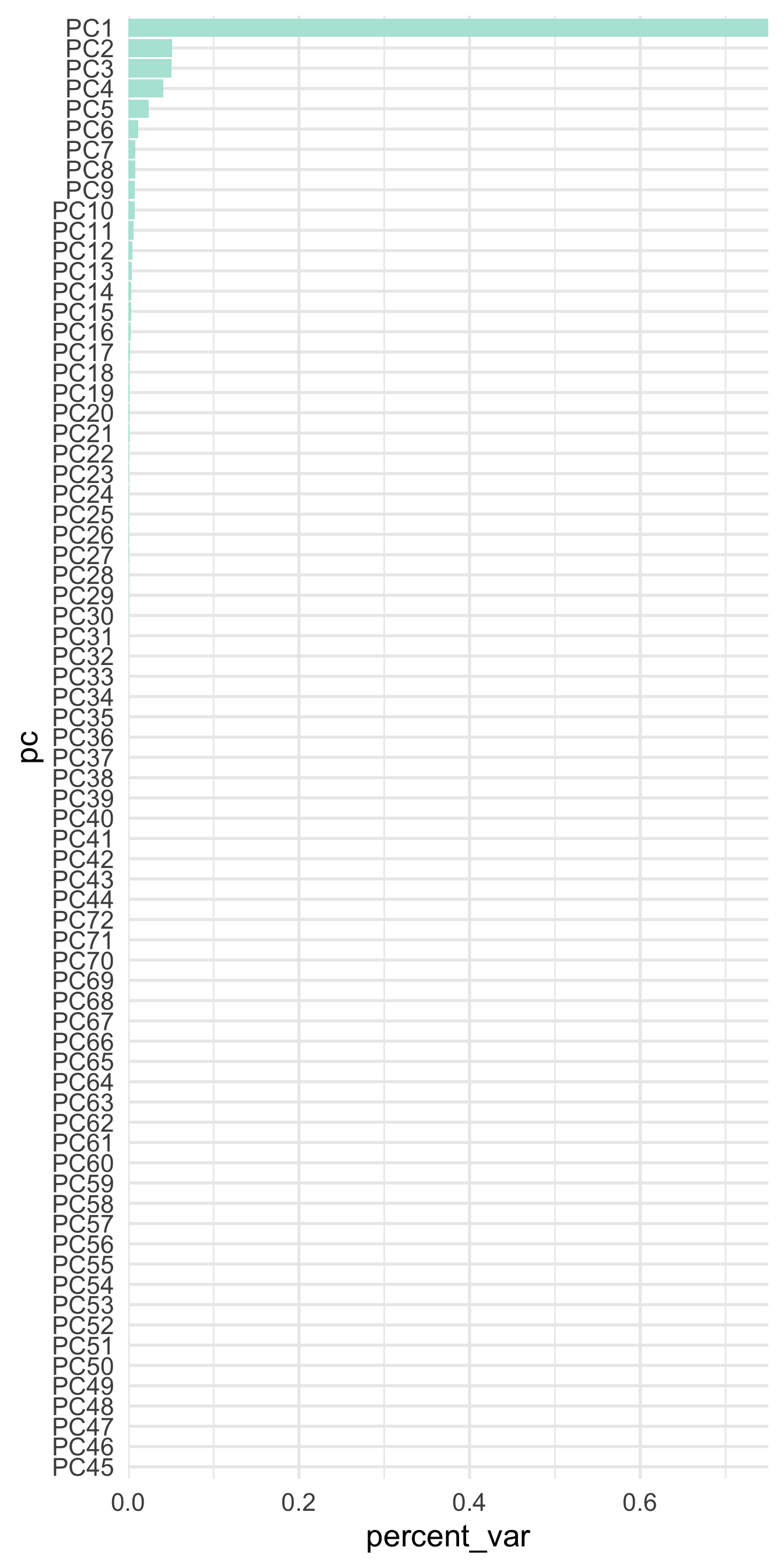
A few things are of note here. First, it appears the majority of the variance is accounted for by our first few components, which is not altogether surprising given that we already new the first 10 components accounted for approximately 85% of the total variability. However, you might also wonder why there are so many freaking components shown?! I thought we only asked for five!? That is true. But the model actually estimates all the components, and then just pulls out whatever we ask, based on either the threshold or the num_comp arguments. For example, let’s bake the five component recipe on the full training data and print the resulting variables.
##  [1] "id"                  "attnd_dist_inst_id"  "attnd_schl_inst_id"
##  [4] "tst_dt"              "partic_dist_inst_id" "partic_schl_inst_id"
##  [7] "ncessch"             "score"               "PC1"
## [10] "PC2"                 "PC3"                 "PC4"
## [13] "PC5"
And as expected, we get only the five components we requested.
PCA reduces the dimensionality in the data, which can help guard against overfitting. However, it also may introduce a small amount of bias. Plots like the above can help determine how many components we should retain because we can see that, for example, after about 20 components or so we’re getting almost nothing in return. If you are using PCA and your model still seems to be overfitting, try reducing the dimensionality more (extracting fewer components). On the other hand, if you do not appear to be in danger of overfitting, you might try extracting more components to help reduce bias.
31.10 Wrapping up
Feature engineering is a gigantic topic. The purpose of this chapter was to provide a basic introduction. We illustrated creating a recipe or blueprint for your feature engineering, which can be applied iteratively to slices of the data (as in a k-fold cross-validation approach) or to new data with the same structure. This process helps guard against data leakage, where information from the test set leaks into the training set. Let’s look at a quick example of this by using PCA to retain 95% of the total variation in the data. We’ll use \(k\)-fold cross-validation and see how many components we retain in each fold. First, we’ll create the recipe, which is essentially equivalent to what we saw in the previous chapter.
rec <- recipe(score ~ ., train) %>%
  step_mutate(tst_dt = lubridate::mdy_hms(tst_dt)) %>%
  update_role(contains("id"), ncessch, new_role = "id vars") %>%
  step_zv(all_predictors()) %>%
  step_unknown(all_nominal()) %>%
  step_medianimpute(all_numeric(), -all_outcomes(), -has_role("id vars")) %>%
  step_normalize(all_numeric(), -all_outcomes(), -has_role("id vars")) %>%
  step_dummy(all_nominal(), -has_role("id vars")) %>%
  step_pca(all_numeric(), -all_outcomes(), -has_role("id vars"),
           threshold = .95)
Now let’s create our \(k\)-fold cross-validation object.
## #  10-fold cross-validation
## # A tibble: 10 x 2
##    splits             id
##    <list>             <chr>
##  1 <split [2.6K/285]> Fold01
##  2 <split [2.6K/284]> Fold02
##  3 <split [2.6K/284]> Fold03
##  4 <split [2.6K/284]> Fold04
##  5 <split [2.6K/284]> Fold05
##  6 <split [2.6K/284]> Fold06
##  7 <split [2.6K/284]> Fold07
##  8 <split [2.6K/284]> Fold08
##  9 <split [2.6K/284]> Fold09
## 10 <split [2.6K/284]> Fold10
Now we’ll loop through each split and pull out the data we will build our model on, for that fold.
## #  10-fold cross-validation
## # A tibble: 10 x 3
##    splits             id     assessment_data
##    <list>             <chr>  <list>
##  1 <split [2.6K/285]> Fold01 <tibble [285 × 39]>
##  2 <split [2.6K/284]> Fold02 <tibble [284 × 39]>
##  3 <split [2.6K/284]> Fold03 <tibble [284 × 39]>
##  4 <split [2.6K/284]> Fold04 <tibble [284 × 39]>
##  5 <split [2.6K/284]> Fold05 <tibble [284 × 39]>
##  6 <split [2.6K/284]> Fold06 <tibble [284 × 39]>
##  7 <split [2.6K/284]> Fold07 <tibble [284 × 39]>
##  8 <split [2.6K/284]> Fold08 <tibble [284 × 39]>
##  9 <split [2.6K/284]> Fold09 <tibble [284 × 39]>
## 10 <split [2.6K/284]> Fold10 <tibble [284 × 39]>
And finally, we’ll apply the recipe to each dataset.
cv %>%
  mutate(assessment_data = map(splits, assessment),
         baked_data = map(assessment_data, ~prep(rec) %>%  bake(.x)))
## # 10-fold cross-validation
## # A tibble: 10 x 4
## splits id assessment_data baked_data
## <list> <chr> <list> <list>
## 1 <split [2.6K/285]> Fold01 <tibble [285 × 39]> <tibble [285 × 17]>
## 2 <split [2.6K/284]> Fold02 <tibble [284 × 39]> <tibble [284 × 17]>
## 3 <split [2.6K/284]> Fold03 <tibble [284 × 39]> <tibble [284 × 17]>
## 4 <split [2.6K/284]> Fold04 <tibble [284 × 39]> <tibble [284 × 17]>
## 5 <split [2.6K/284]> Fold05 <tibble [284 × 39]> <tibble [284 × 17]>
## 6 <split [2.6K/284]> Fold06 <tibble [284 × 39]> <tibble [284 × 17]>
## 7 <split [2.6K/284]> Fold07 <tibble [284 × 39]> <tibble [284 × 17]>
## 8 <split [2.6K/284]> Fold08 <tibble [284 × 39]> <tibble [284 × 17]>
## 9 <split [2.6K/284]> Fold09 <tibble [284 × 39]> <tibble [284 × 17]>
## 10 <split [2.6K/284]> Fold10 <tibble [284 × 39]> <tibble [284 × 17]>Let’s see how many principal components are in each data fold.
cv %>%
  mutate(assessment_data = map(splits, assessment),
         baked_data = map(assessment_data, ~prep(rec) %>%  bake(.x)),
         n_components = map_int(baked_data, ~sum(grepl("^PC", names(.x)))))
## # 10-fold cross-validation
## # A tibble: 10 x 5
## splits id assessment_data baked_data n_components
## <list> <chr> <list> <list> <int>
## 1 <split [2.6K/285]> Fold01 <tibble [285 × 39]> <tibble [285 × 17… 9
## 2 <split [2.6K/284]> Fold02 <tibble [284 × 39]> <tibble [284 × 17… 9
## 3 <split [2.6K/284]> Fold03 <tibble [284 × 39]> <tibble [284 × 17… 9
## 4 <split [2.6K/284]> Fold04 <tibble [284 × 39]> <tibble [284 × 17… 9
## 5 <split [2.6K/284]> Fold05 <tibble [284 × 39]> <tibble [284 × 17… 9
## 6 <split [2.6K/284]> Fold06 <tibble [284 × 39]> <tibble [284 × 17… 9
## 7 <split [2.6K/284]> Fold07 <tibble [284 × 39]> <tibble [284 × 17… 9
## 8 <split [2.6K/284]> Fold08 <tibble [284 × 39]> <tibble [284 × 17… 9
## 9 <split [2.6K/284]> Fold09 <tibble [284 × 39]> <tibble [284 × 17… 9
## 10 <split [2.6K/284]> Fold10 <tibble [284 × 39]> <tibble [284 × 17… 9In this case, the number of components is the same across all folds, but the representation of those components is likely slightly different. Why? Because the recipe has been applied to each fold, independent of the other folds.
Feature engineering can also regularly feel overwhelming. There are so many possible options that you could do to potentially increase model performance. This chapter just scratched the surface. The sheer number of decisions is why many believe that feature engineering is the most “art” part of machine learning. Strong domain knowledge will absolutely help, as will practice. For those looking to go further with feature engineering, we suggest Kuhn and Johnson, who wrote an entire book on the topic. It provides practical advice in an accessible way without skimping on important details.