35 Boosting and Boosted Trees
Similar to bagging, boosting is a general algorithm that can be applied to any model. Frequently, however, it is applied to trees. Recall that when we use bagging (often through bagged tree or random forest models), we needed to have a sufficient number of bags, or bootstrap resamples, of the training data so our model performance metrics stabilize. Including additional bags (trees) once the performance has stabilized will not hurt in terms of model performance, but it will take longer to fit (i.e., more computationally expensive).
Similar to bagging, boosting works by building an ensemble of models. However, rather than each model being built independently on a new bootstrap resample of the original data, the subsequent models are constructed from the residuals of the previous model. This means that the number of models used controls how much is learned from the data and is an important hyperparameter.
Boosting versus Bagging
Bagged models use \(b\) bootstrap resamples of the training data. Models are built independently on each resample, and model results are aggregated to form a single prediction
Boosted models are built sequentially, with each model fit to the residuals of the previous model
For bagged models, \(b\) needs to be sufficiently large that performance metrics stabilize. Additional bags beyond this point only hurt computational efficiency.
For boosted models, the number of models determines how much is learned from the data: too few, and the model will underfit (leading to excess bias), too many and the model will overfit (leading to excess variance).
The model that is iteratively fit when applying boosting is called the base learner. This can be any model but is regularly a decision tree because, in part, it is relatively straightforward to control how much each individual tree learns from the data (i.e., shallow trees will learn less from the data than deeper trees).
Base learner: The model that is iteratively fit within a boosting algorithm. Often these are shallow decision trees, as in a boosted tree model.
Weak models & slow learning: Each model builds off the errors of the previous model. To find an optimal solution, we want our base learner to learn slowly, so the amount that is learned is controlled by the number of models.
We also typically want our base learner to be a weak model, otherwise known as a slow learner. Imagine, for example, that you were wearing a blindfold in a meadow with many small hills. Some are as high as ten feet above where you are currently, while other dip beneath you up to about five feet. You are challenged to find the lowest point in the valley, while remaining blindfolded. You are given an additional directive that the size of your step must be the same each time. If you take off at a sprint you may, beyond falling on your face, accidentally skip right over the lowest point because the length of your stride would be sufficient to carry you over. Further, you would not even be able to get to the lowest point, because each subsequent stride may carry you over again (remember, each stride must be the same length). This is equivalent to a model that learns fast. You would likely get close quickly (running downhill), but your final solution may not be optimal.
If, on the other hand, you take smaller, more careful steps, it would take you longer to get to the lowest point, but your stride would be less likely to carry you over the lowest point, and you would be able to feel when the gradient beneath you steepens. This does not guarantee you’ll find the lowest point, of course, but there’s probably a better chance than you’d have if you were sprinting. This is the idea behind a slow learner. We take more steps (number of models we fit), but each gets us closer to the optimal solution.
How do we determine what’s optimal? We us our objective function, along with a process called gradient descent. Our objective function tells us the criteria that we want to minimize or maximize. We can, theoretically, evaluate the objective function for any model parameters. We use gradient descent to optimize the model parameters with respect to the objective function (which we maximize or minimize).
35.1 Gradient descent
Gradient descent is a general purpose optimization algorithm that is used (or most frequently, a variant is used) throughout many machine learning applications. When thinking about gradient descent conceptually, the scenario described previously of walking around a meadow blindfolded is again useful. If we were trying to find the lowest point, we would probably feel around us and find the direction that seemed the steepest. We would then take a step in that direction. If we were being careful, we would check the ground around us again after each step, evaluating the gradient immediately around us, and then continuing on in the steepest direction. This is the basic idea of gradient descent. We start off in a random location on some surface, and we step in the steepest direction until we can’t go down any further.
Consider a simple example with a linear regression model. First, let’s simulate some data.
set.seed(42)
n <- 1000
x <- rnorm(n)

a <- 5
b <- 1.3
e <- 4

y <- a + b*x + rnorm(n, sd = e)

sim_d <- tibble(x = x, y = y)

ggplot(sim_d, aes(x, y)) +
geom_point() 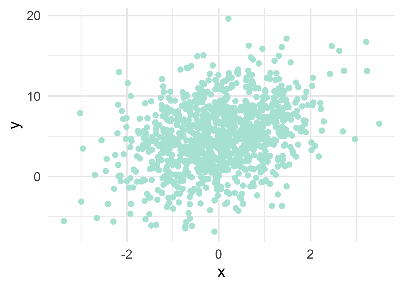
We can estimate the relation between \(x\) and \(y\) using standard OLS, as follows:
##
## Call:
## lm(formula = y ~ x)
##
## Residuals:
##      Min       1Q   Median       3Q      Max
## -11.6899  -2.6353  -0.0333   2.6513  14.3506
##
## Coefficients:
##             Estimate Std. Error t value Pr(>|t|)
## (Intercept)   4.9797     0.1248   39.89   <2e-16 ***
## x             1.3393     0.1245   10.75   <2e-16 ***
## ---
## Signif. codes:  0 '***' 0.001 '**' 0.01 '*' 0.05 '.' 0.1 ' ' 1
##
## Residual standard error: 3.946 on 998 degrees of freedom
## Multiple R-squared:  0.1039, Adjusted R-squared:  0.103
## F-statistic: 115.7 on 1 and 998 DF,  p-value: < 2.2e-16
This not only provides us the best linear unbiased estimate (BLUE) of the relation between \(x\) and \(y\), but it is computed extremely fast (around a tenth of a second on my computer).
Let’s see if we can replicate these values using gradient descent. We will be estimating two parameters, the intercept and the slope of the line (as above). Our objective function is the mean squared error. That is, we want to find the line running through the data that minimizes the average distance between the line and the points. In the case of simple linear regression, the mean square error is defined by
\[ \frac{1}{N} \sum_{i=1}^{n} (y_i - (a + bx_i ))^2 \]
where \(a\) is the intercept of the line and \(b\) is the slope of the line. Let’s write a function in R that computes the mean square error for any line.
mse <- function(a, b, x = sim_d$x, y = sim_d$y) {
  prediction <- a + b*x # model prediction, given intercept/slope
  residuals <- y - prediction # distance between prediction & observed
  squared_residuals <- residuals^2 # squared to avoid summation to zero
  ssr <- sum(squared_residuals) # sum of squared distances

  mean(ssr) # average of squared distances
}
Notice in the above we pre-defined the x and the y values to be from our simulated data, but the function is general enough to compute the mean squared error for any set of data.
Just to confirm that our function works, let’s check that our MSE with the OLS coefficients matches what we get from the model.
## [1] 15539.95Is this the same thing we get if we compute it from the model residuals?
## [1] 15539.95It is!
So now we have a general function that can be used to evaluate our objective function for any intercept/slope combination. We can then, theoretically, evaluate infinite combinations and find the lowest value. Let’s look at several hundred combinations.
# candidate values
grid <- expand.grid(a = seq(-5, 10, 0.1), b = seq(-5, 5, 0.1)) %>%
  as_tibble()
grid
## # A tibble: 15,251 x 2
## a b
## <dbl> <dbl>
## 1 -5 -5
## 2 -4.9 -5
## 3 -4.8 -5
## 4 -4.7 -5
## 5 -4.6 -5
## 6 -4.5 -5
## 7 -4.4 -5
## 8 -4.3 -5
## 9 -4.2 -5
## 10 -4.1 -5
## # … with 15,241 more rowsWe could, of course, overlay all of these on our data, but that would be really difficult to parse through with 15,251 candidate lines. Let’s compute the MSE for each candidate.
## # A tibble: 15,251 x 3
##        a     b     mse
##    <dbl> <dbl>   <dbl>
##  1  -5      -5 152243.
##  2  -4.9    -5 150290.
##  3  -4.8    -5 148357.
##  4  -4.7    -5 146444.
##  5  -4.6    -5 144551.
##  6  -4.5    -5 142677.
##  7  -4.4    -5 140824.
##  8  -4.3    -5 138991.
##  9  -4.2    -5 137178.
## 10  -4.1    -5 135384.
## # … with 15,241 more rows
Let’s actually look at this grid
Notice this is basically just a big valley because this is a very simple (and linear) problem. We want to find the combination that minimizes the MSE which, in this case, is:
## # A tibble: 1 x 3
##       a     b    mse
##   <dbl> <dbl>  <dbl>
## 1     5   1.3 15542.
How does this compare to what we estimated with OLS?
## (Intercept)           x
##    4.979742    1.339272
Pretty similar.
But this still isn’t gradient descent. This is basically just a giant search algorithm that is only feasible because the problem is so simple.
So what is gradient descent and how do we implement it? Conceptually, it’s similar to our blindfolded walk - we start in a random location and try to walk downhill until we get to what we think is the lowest point. A more technical description is given in the box below.
Gradient Descent
- Define a cost function (such as MSE).
- Calculate the partial derivative of each parameter of the cost function. These provide the gradient (steepness), and the direction the algorithm needs to “move” to minimize the cost function.
- Define a learning rate. This is the size of the “step” we take downhill.
- Multiply the learning rate by the partial derivative value (this is how we actually “step” down).
- Estimate a new gradient and continue iterating (\(\text{gradient} \rightarrow \text{step} \rightarrow \text{gradient} \rightarrow \text{step} \dots\)) until no further improvements are made.
Let’s try applying gradient descent to our simple linear regression problem. First, we have to take the partial derivative of each parameter, \(a\) and \(b\), for our cost function. The is defined as
\[ \begin{bmatrix} \frac{d}{da}\\ \frac{d}{db}\\ \end{bmatrix} = \begin{bmatrix} \frac{1}{N} \sum -2(y_i - (a + bx_i)) \\ \frac{1}{N} \sum -2x_i(y_i - (a + bx_i)) \\ \end{bmatrix} \]
Let’s write a function to calculate the gradient (partial derivative) for any values of the two parameters. Similar to the mse() function we wrote, we’ll define this assuming the sim_d data, but have it be general enough that other data could be provided.
compute_gradient <- function(a, b, x = sim_d$x, y = sim_d$y) {
  n <- length(y)
  predictions <- a + (b * x)
  residuals <- y - predictions

  da <- (1/n) * sum(-2*residuals)
  db <- (1/n) * sum(-2*x*residuals)

  c(da, db)
}
Great! Next, we’ll write a function that uses the above function to calculate the gradient, but then actually takes a step in that direction. We do this by first multiplying our partial derivatives by our learning rate (the size of each step) and then subtracting that value from whatever the parameters are currently. We subtract because we’re trying to go “downhill”. If we were trying to maximize our objective function, we would add these values to our current parameters (technically gradient ascent).
Learning rate defines the size of the step we take downhill. Higher learning rates will get us closer to the optimal solution faster, but may “step over” the minimum. When training a model, start with a relatively high learning rate (e.g., \(0.1\)) and adjust as needed. Before finalizing your model, consider reducing the learning rate to ensure you’ve found the global minimum.
gd_step <- function(a, b,
                    learning_rate = 0.1,
                    x = sim_d$x,
                    y = sim_d$y) {
  grad <- compute_gradient(a, b, x, y)
  step_a <- grad[1] * learning_rate
  step_b <- grad[2] * learning_rate

  c(a - step_a, b - step_b)
}
And finally, we choose a random location to start, and begin our walk! Let’s begin at 0 for each parameter.
## [1] 0.9890313 0.2433964After just a single step, our parameters have changed quite a bit. Remember that our true values are 5 and 1.3. Both parameters appear to be heading in the right direction. Let’s take a few more steps. Notice that in the below we’re taking a step from the previous location.
## [1] 1.7815134 0.4429925## [1] 2.4165300 0.6065743## [1] 2.9253881 0.7405655Our parameters continue to head in the correct direction. However, the amount that the values change gets less with each iteration. This is because the gradient is less steep. So our “stride” is not carrying us as far, even though the size of our step is the same.
Let’s speed this up a bit (although you could continue on to “watch” the parameters change) by using a loop to quickly take 25 more steps downhill.
## [1] 4.971523 1.335808And now we are very close! What if we took 25 more steps?
## [1] 4.979709 1.339254We get almost exactly the same thing. Why? Because we were already basically there. If we continue to try to go downhill we just end up walking around in circles.
Let’s rewrite our functions a bit to make the results a little easier to store and inspect later.
estimate_gradient <- function(pars_tbl, learning_rate = 0.1, x = sim_d$x, y = sim_d$y) {

  pars <- gd_step(pars_tbl[["a"]], pars_tbl[["b"]],
                  learning_rate)

  tibble(a = pars[1], b = pars[2], mse = mse(a, b, x, y))
}

# initialize
grad <- estimate_gradient(tibble(a = 0, b = 0))

# loop through
for(i in 2:50) {
  grad[i, ] <- estimate_gradient(grad[i - 1, ])
}
grad
## # A tibble: 50 x 3
## a b mse
## <dbl> <dbl> <dbl>
## 1 0.989 0.243 32446.
## 2 1.78 0.443 26428.
## 3 2.42 0.607 22552.
## 4 2.93 0.741 20057.
## 5 3.33 0.850 18450.
## 6 3.66 0.940 17415.
## 7 3.92 1.01 16748.
## 8 4.13 1.07 16318.
## 9 4.30 1.12 16042.
## 10 4.43 1.16 15863.
## # … with 40 more rowsFinally, let’s add our iteration number into the data frame, and plot it.
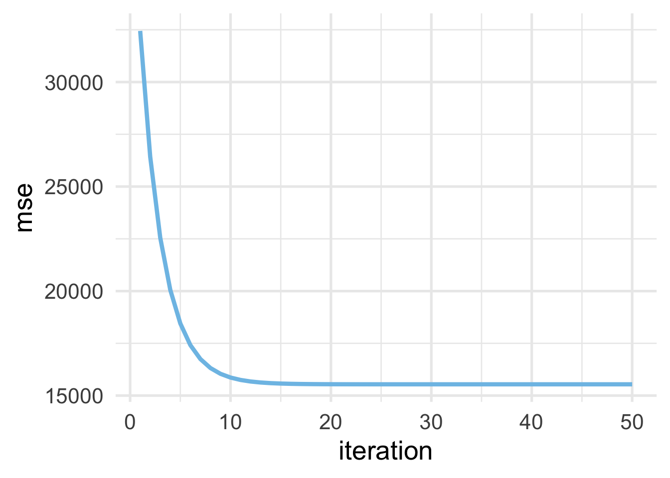
As we would expect, the MSE drops very quickly as we start to walk downhill (with each iteration) but eventually (around 20 or so iterations) starts to level out when no more progress can be made.
Let’s look at this slightly differently. by looking at our cost surface, and how we step down the cost surface.
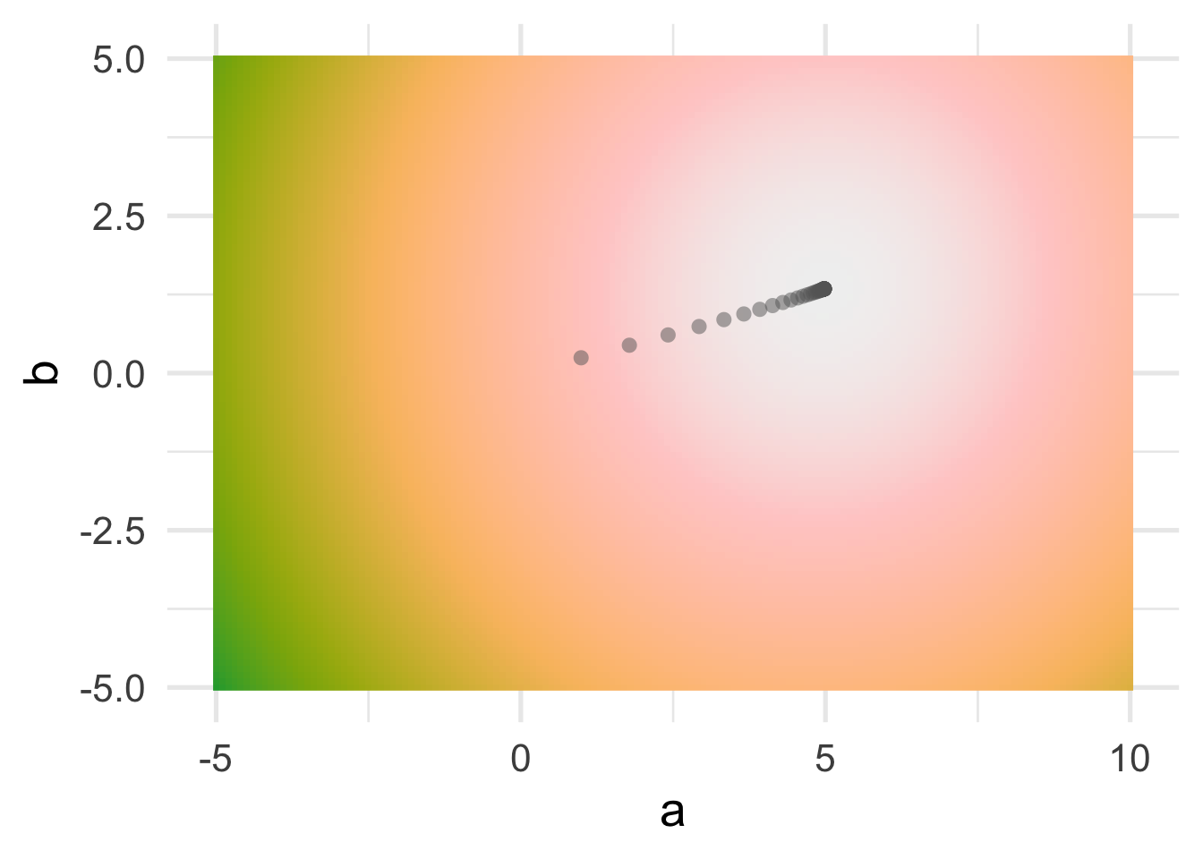
You can see that, as we would expect, the algorithm takes us straight “downhill”.
Finally, because this is simple linear regression, we can also plot out the line through the iterations (as the algorithm “learns” the optimal intercept/slope combination).
ggplot(sim_d, aes(x, y)) +
  geom_point() +
  geom_abline(aes(intercept = a, slope = b),
              data = grad,
              color = "gray60",
              size = 0.3) +
  geom_abline(aes(intercept = a, slope = b),
              data = grad[nrow(grad), ],
              color = "magenta")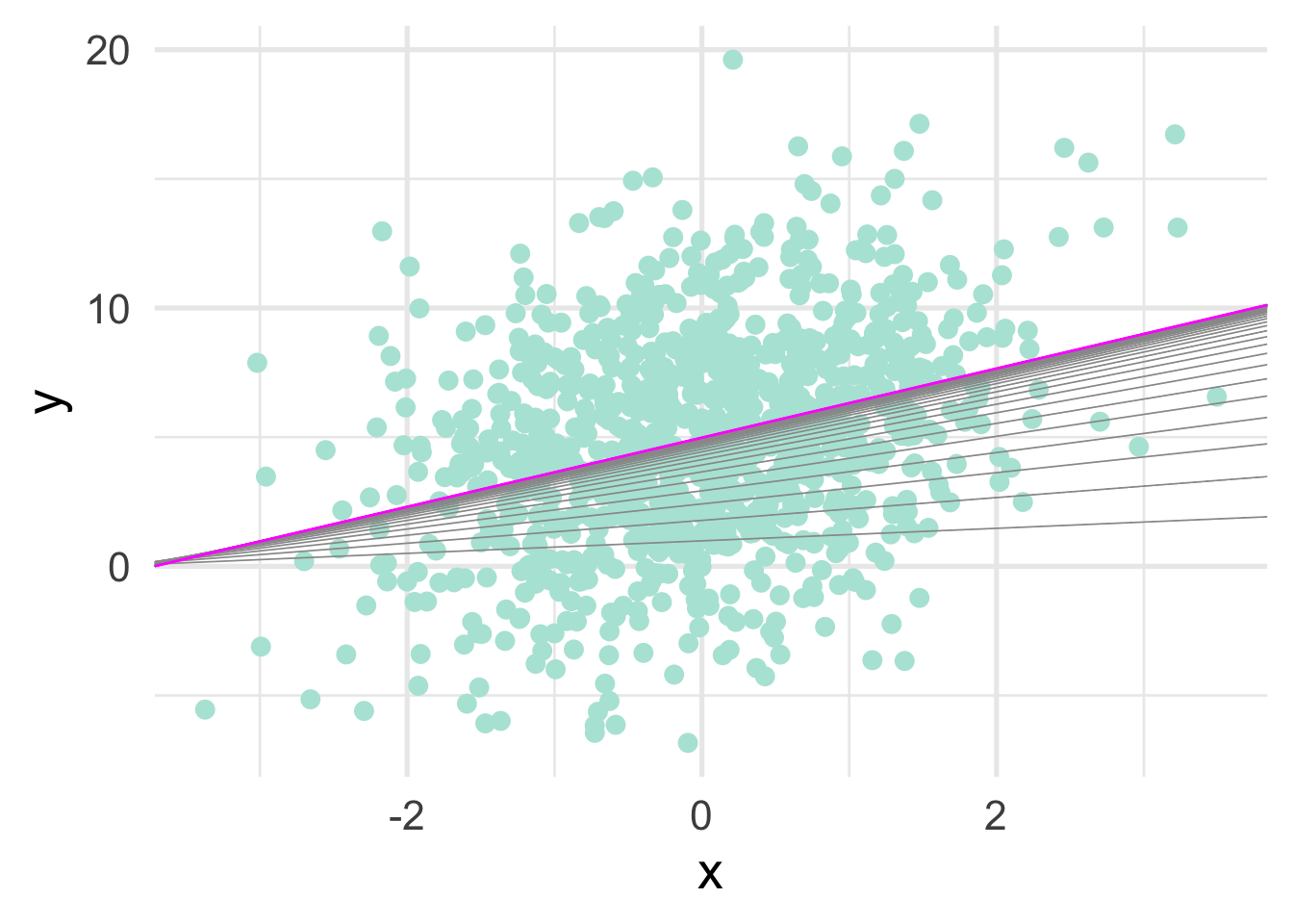
Or, just for fun, we could animate it.
library(gganimate)
ggplot(grad) +
  geom_point(aes(x, y), sim_d) +
  geom_smooth(aes(x, y), sim_d,
              method = "lm", se = FALSE) +
  geom_abline(aes(intercept = a,
                  slope = b),
              color = "#de4f60") +
  transition_manual(frames = iteration)
## NULLSo in the end, gradient descent gets us essentially the exact same answer we get with OLS. So why would we use this approach instead? Well, if we’re estimating a model with something like regression, we wouldn’t. As is probably apparent, this approach is going to be more computationally expensive, particularly if we have a poor starting location. But in many cases we don’t have a closed-form solution to the problem. This is where gradient descent (or a variant thereof) can help. In the case of boosted trees, we start by building weak model with only a few splits (including potentially only one). We then build a new (weak) model from the residuals of this model, using gradient descent to optimize each split in the tree relative to the cost function. This ensures that our ensemble of trees builds toward the minimum (or maximum) of our cost function.
As is probably clear, however, gradient descent is a fairly complicated topic. We chose to focus on a relatively “easy” implementation within a simple linear regression framework, which has only two parameters. There are a number of potential pitfalls related to gradient descent, including exploding gradients, where the search algorithm gets “lost” and basically wanders out into space. This can happen if the learning rate is too high. Normalizing your features so they are all on a common scale can also help prevent exploding gradients. Vanishing gradients is a similar problem, where the gradient is small enough that the new parameters do not change much and the algorithm gets “stuck”. This is okay (and expected) if the algorithm has reached the global minimum, but is a problem if it’s only at a local minimum (i.e., stuck in a valley on a hill). There are numerous variants of gradient descent that can help with these challenges, as we will discuss in subsequent chapters.
35.2 Boosted trees
Like all boosted models, boosted trees are built with weak models so the overall algorithm learns slowly. We want the model to learn slowly so that it can pick up on the unique characteristics of the data and find the overall optimal solution. If it learns too quickly it may “jump over” the optimal solution.
In the feature engineering chapter, we discussed methods for handling things like nonlinearity through, for example, splines. When working through a linear regression framework, splines can create smooth curves that model any non-linear relations. Recall, however, that decision trees work by splitting the feature space into distinct regions. In other words, decision trees do not, by themselves, create curves. But if the model learns slowly enough it is possible to approximate curves, non-parametrically, even if we do not know the underlying functional form of the data a priori.
For example, the figure below shows a boosted tree model fit to the same log data we saw previously using 1, 5, 50, 100, 200 and 500 trees.
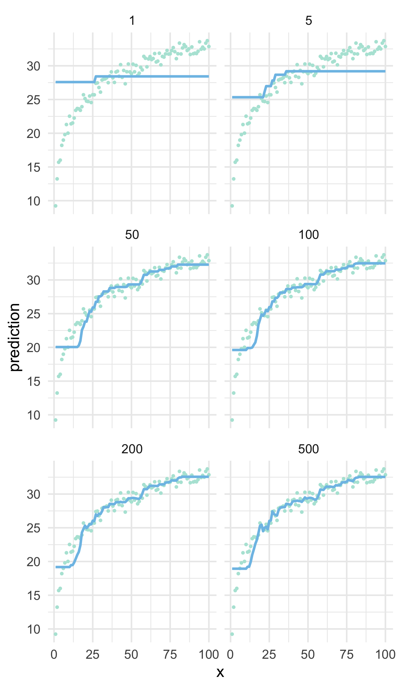
Initially, the errors (average distance between a point the line) are extremely high. But as more trees are built from the residuals of the previous, the algorithm starts to learn the underlying functional form. Note that this is still not as good as what we would get if we just log transformed the \(x\) variable and fit a simple linear regression model because, of course, that is how the data were generated. Once we get to 500 trees we could argue that the model is starting to overfit in some regions, while still badly underfitting at the bottom tail. This is an important example of the no free lunch theorem where, in this case, we have fit a relatively advanced machine learning model to a simple set of data, the results of which would be easily outperformed by simple linear regression. No single model will always work best across all applications. However, with proper hyperparameter tuning, boosted decision trees are regularly among the most performant “out of the box”.
35.2.1 Hyperparameters and engines
Standard boosted tree hyperparameters
- Number of trees
- Number of splits for each tree
- Minimum \(n\) size for a terminal node
- Learning rate
We have talked about each of the hyperparameters listed above previously. However, it’s worth thinking more about how they work together in a boosted tree model.
Generally, the minimum sample size for a terminal node will not factor in heavily with boosted tree models, because the trees are typically grown quite shallow (so the model learns slowly). The number of splits is often between one (a stump) and six, although occasionally models with deeper trees can work well. The depth of the tree (generally controlled more heavily by the number of splits than the terminal \(n\) size) will determine the number of trees needed to arrive at an optimal solution. Deeper trees will learn more from the data, and will therefore generally require fewer trees. Deeper trees also allow for interactions among variables - i.e., the splits are conditional on previous splits, and thus the prediction depends on the interaction among the features in the tree. If important interactions in the data exist, the trees will need to be grown to a sufficient depth to capture them. An ensemble of stumps (trees with just a single split) are relatively common and computationally efficient, although they do generally require more trees, as each tree learn very little about the data (as illustrated above). Because they learn more slowly, they are less likely to overfit. These models will, however, miss any interactions that may be present in the data.
Standard boosted tree tuning strategy
- Set learning rate around \(0.1\)
- Tune the number of trees
- Fix the number of trees, tune number of splits (and potentially minimum terminal \(n\) size)
- Fix tree depth & terminal \(n\), tune learning rate
- Fix all other hyperparameters, evaluate the number of trees again. If (more than marginally) different, set the number of trees to the new value and continue tuning.
The learning rate is a new parameter that we haven’t seen with any tree-based model previously (although we also didn’t have to tune the number of trees previously, we just had to make sure we had a sufficient number to reach a stable estimate). We talked about the learning rate some in the section on gradient descent but it’s worth reiterating that, along with the number of trees, the learning rate is perhaps the most important hyperparameter. If the learning rate is too high, the model is likely to “jump over” the optimal solution, and if it is too low the model may take far too long to reach an optimal solution. The learning rate is also called the shrinkage parameter because it is the amount by which we multiply the partial derivatives of our cost function (the gradient). Smaller values will result in smaller “steps” downhill, and in turn, the amount each tree learns. As a practical recommendation, we suggest starting with a learning rate around \(0.1\). Values higher than this do not typically work well, in our experience, but it is high enough that the model should find a value close to the minimum relatively fast. Once you’ve conducted your model tuning on the other hyperparameters with this learning rate, consider reducing the learning rate to see if you can increase model performance further (e.g., to values of \(0.01\) or \(0.001\)).
The {gbm} package (for gradient boosted models) is perhaps the most common package for estimating standard boosted trees. Throughout this book, however, we have been been using the {tidymodels} suite of packages and, although multiple boosting engines have been implemented, {gbm} is not one of them. Although it is possible to add new engines or models to {parsnip}, the {gbm} package is in many ways a simpler implementation of boosted models than those that are already implemented in {parsnip}, specifically the {xgboost} package, which includes a number of additional hyperparameters, as follows.
{xgboost} hyperparameters
- Number of trees
- Number of splits for each tree
- Minimum \(n\) size for a terminal node
- Learning rate
- Number of predictors to be randomly sampled at each split
- Proportion of cases to sample for each tree
- Limiting tree depth by the cost function (reduction required to continue splitting the tree)
- Early stopping criteria (stop growing additional trees during training if there is no change in the cost function on the validation set for \(k\) consecutive trees)
As can be seen, the same hyperparameters for standard boosted trees are available when using the {xgboost} engine, but additional stochastic based parameters are also available (randomly sampling columns at each split and cases for each tree). The stochastic parameters are based in the same underlying principles that help improve the performance of bagged trees and random forests. Exposing only a sample of the data and features to the algorithm at a time may make the algorithm take a bit more time, as each tree is likely to learn less (making it learn even more slowly). But it may also pick up on meaningful aspects of the data that are otherwise missed. Of course, the extent to which including these stochastic components helps you model performance will depend on your data. For example, random selection of columns will likely help more when you have a few features that are strongly related to the outcome and many that are weakly related (i.e., so each subsequent tree isn’t built by starting with the same features as the root node).
Tuning {xgboost} models
The early stopping rules change the way we tune our model. We can use a very large number of trees with early stopping to
- Tune the learning rate, then
- Tune tree depth, then
- Evaluate if stochastic components help, then
- Re-tune learning rate
If the cross-validation curve suggests overfitting, include regularization methods (e.g., limiting tree depth by changes in the cost function, L1 or L2 regularizers)
Beyond these additional stochastic-based hyperparameters, {xgboost} provides an alternative method by which tree depth can be limited. Specifically, if the cost function is not reduced below a given threshold, the tree stops growing. Further, when tuning a model, {xgboost} allows for the use of early stopping rule. This works by evaluating changes in the gradient across iterations (trees) on the validation set during training. If no improvements are made after a specified number of trees, then the algorithm stops. Early stopping can provide immense gains in computational efficiency (by not continuing to grow a tree when no improvements are being) while also helping to prevent overfitting. Rather than being an additional parameter to tune, you can use early stopping to your advantage to only fit the number trees necessary, while being adaptive across different model specifications (e.g., tree depth).
The {xgboost} package itself includes even more hyperparameters, including slightly alternative methods for fitting the model altogether. For example, the dart booster includes a random dropout component. The idea, which originated with neural nets, is that trees added early in the ensemble will be more important than trees added late in the ensemble. So, particularly in cases where the model overfits quickly, it can be helpful to randomly remove (drop) specific trees from the overall ensemble. This is a rather extreme regularization approach, but has been shown to improve performance in some situations.
In what follows, we discuss implementation with {tidymodels}. However, we will also provide a few examples with {xgboost} directly, including direct comparisons between the two implementations. Our motivation here is not necessarily to advocate for the use of one versus the other, but to highlight that there are some differences and, depending on your specific situation, you might prefer to use one over the other. For example, if you do not have a need to move outside of the hyperparameters that have already been implementedin {parsnip} for the {xgboost} engine, there’s likely no need to move outside of the {tidymodels} framework. If, however, you are having problems with severe overfitting and you want to try using dropout for regularization, then you will need to move to {xgboost} directly with the dart booster.
35.3 Fitting boosted tree models
Let’s use our same statewide testing data we have now used at numerous points, along with our same recipe.
library(sds)
library(tidyverse)
library(tidymodels)
library(tictoc)

set.seed(41920)
full_train <- get_data("state-test") %>%
  slice_sample(prop = 0.05) %>%
  select(-classification)

splt <- initial_split(full_train)
train <- training(splt)
cv <- vfold_cv(train)
Next we’ll specify a basic recipe. One thing to note about the below is that we generally don’t have to worry about dummy-coding variables for decision trees. However, dummy-coding (or one-hot encoding) is necessary when using {xgboost}.
rec <- recipe(score ~ ., train) %>%
  step_mutate(tst_dt = as.numeric(lubridate::mdy_hms(tst_dt))) %>%
  update_role(contains("id"), -ncessch, new_role = "id vars") %>%
  step_zv(all_predictors()) %>%
  step_novel(all_nominal()) %>%
  step_unknown(all_nominal()) %>%
  step_medianimpute(all_numeric(),
                    -all_outcomes(),
                    -has_role("id vars"))  %>%
  step_dummy(all_nominal(),
             -has_role("id vars"),
             one_hot = TRUE) %>%
  step_nzv(all_predictors(), freq_cut = 995/5)
XGBoost is “an optimized distributed gradient boosting library designed to be highly efficient” (emphasis in the original, from the XGBoost documentation). The distributed part means that the models are built to work efficiently with parallel processing, and is (relative to alternative methods) extremely fast. We specify the model the same basic way we always do in the {tidymodels} framework, using parsnip::boost_tree() to specify the model and setting the engine to xgboost. We’ll also set the mode to be regression.
We can translate this model to essentially a raw {xgboost} model using the translate function.
## Boosted Tree Model Specification (regression)
##
## Computational engine: xgboost
##
## Model fit template:
## parsnip::xgb_train(x = missing_arg(), y = missing_arg(), nthread = 1,
##     verbose = 0)
Note that the data have not yet been specified (we pass these arguments when we use fit_resamples() or similar). Additionally, the nthread argument specifies the number of processors to use in parallel processing. By default, {parsnip} sets this argument to 1, but {xgboost} will set it to the maximum number of processors available. We can change this by passing the nthread argument either directly to set_engine() or to set_args().
Additionally, we want to use early stopping. To do this we have to pass three additional arguments: ntree, stop_iter and validation. These arguments represent, respectively, the maximum number of trees to use, the number of consecutive trees that should show no improvement on the validation set to exit the stop the algorithm, and the proportion of the data that should be used for the validation set (to monitor the objective function and potentially exit early). The maximum number of trees should just be sufficiently large that early stopping will kick in at some point. The stop_iter argument is a hyperparameter, but is less important than other - generally we use somewhere between 20-50, but values of 100 or so may also work well (because they are evaluated against the validation set, generally you just need a number that is sufficiently large). Finally, you must also pass a validation argument specifying the proportion of the data you would like to use to determine early stopping or the early stopping will not work (because it can’t evaluate changes against a validation set when no validation set exists, and there is no default value for validation). We typically use 20% for validation. Additionally it is worth noting that, at least at present, the methods for establishing early stopping differ somewhat between the two implementations (see here).
Let’s specify our model with these additional arguments, while setting the nthread to the maximum.
## [1] 3And finally, we can estimate using the default hyperparameter values.
## 25.956 sec elapsedNotice we’re only working with 5% of the overall sample (to save time in rendering this chapter). But this was relatively quick for 10-fold CV. How does the default performance look?
## # A tibble: 2 x 5
##   .metric .estimator   mean     n std_err
##   <chr>   <chr>       <dbl> <int>   <dbl>
## 1 rmse    standard   89.5      10  1.28
## 2 rsq     standard    0.418    10  0.0134
Not bad! But there’s a lot of tuning we can still do to potentially improve performance from here. Notice that this took 16.8 seconds. What if we do this same thing with {xgboost} directly?
First, we’ll need to process our data
Next, we’re going to drop the ID variables and the outcome and transform the data frame into a matrix, which is what {xgboost} will want.
And now we can fit the model using these data directly with {xgboost}. We’ll still use 10-fold cross-validation, but have {xgboost} do it for us directly. Notice in the below that some of the arguments are a bit different, but they all walk directly to what we used with {tidymodels}. We’re using the squared errors as the objective function, which is equivalent to the mean squared error. Notice also that I do not have specify the nthread argument because it will default to the maximum number of processors.
library(xgboost)
tic()
fit_default_xgb <- xgb.cv(
  data = features,
  label = processed_train$score,
  nrounds = 5000, # number of trees
  objective = "reg:squarederror",
  early_stopping_rounds = 20,
  nfold = 10,
  verbose = FALSE
)
toc(log = TRUE)
## 10.61 sec elapsedAnd this took 25.96 to fit, so just a bit faster. But, this also takes additional time before estimation in data processing (and that data processing happens directly with the {tidymodels} implementation.
How do the results compare? When using {xgboost} directly, the history of the model is stored in an evaluation_log data frame inside the returned object. There is also a best_iteration value that specifies which iteration had the best value for the objective function for the given model. We can use these together to look at our final model results.
##    iter train_rmse_mean train_rmse_std test_rmse_mean test_rmse_std
## 1:   22        78.28245      0.4560459       88.80643       2.20707
And as you can see, the RMSE value for the validation set is very similar to what we got with {tidymodels}.
One nice feature about using {xgboost} directly is that we can use the evaluation_log to plot the learning curve. We just have to first rearrange the data frame a bit.
log_def <- fit_default_xgb$evaluation_log %>%
  pivot_longer(-iter,
               names_to = c("set", "metric", "measure"),
               names_sep = "_") %>%
  pivot_wider(names_from = "measure",
              values_from = "value")
log_def
## # A tibble: 84 x 5
## iter set metric mean std
## <dbl> <chr> <chr> <dbl> <dbl>
## 1 1 train rmse 1753. 0.246
## 2 1 test rmse 1753. 2.79
## 3 2 train rmse 1230. 0.157
## 4 2 test rmse 1230. 2.79
## 5 3 train rmse 864. 0.109
## 6 3 test rmse 864. 2.70
## 7 4 train rmse 609. 0.0808
## 8 4 test rmse 609. 2.60
## 9 5 train rmse 431. 0.0666
## 10 5 test rmse 431. 2.45
## # … with 74 more rowsAnd then we can plot the test and train curves together.
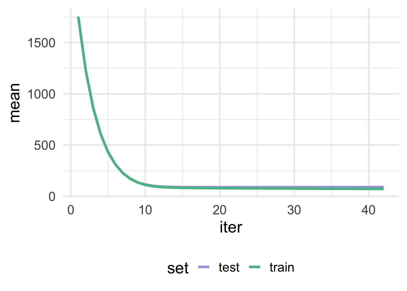
As we can see, in this case, there is very little separation between the test and train sets, which is a good thing. If the curves started to converge but then separated again, or never really converged but always had a big gap between them, this would be strong evidence that we were overfitting (i.e. the training error continues to go down as the test/validation error goes up).
35.3.1 Model tuning
Let’s now tune our model, starting with the learning rate. In what follows, we illustrate this approach using both the {tidymodels} implementation and {xgboost} directly. However, following tuning our model, we proceed with further tuning using only the {tidymodels} implementation.
The models here take a long time to fit. In fact, we did not estimate them here directly. Rather, we sampled half of the total data (rather than 5% as above) and ran each of the models below using a high performance computing cluster. We recommend not running these models on your local computer, and instead using high-performance computing.
First, we need to specify a grid of values to search over. Remember, smaller learning rate values will lead to the model learning slower (and thus taking longer to fit) and risk finding local minima. However, lower learning rates are also more likely to find the global minimum. Higher learning rates will fit quicker, taking larger steps downhill, but risk “stepping over” the global minimum.
First, let’s create a grid of 20 learning rate values to evaluate.
We’ll start with the {tidymodels} approach. Let’s update our previous {parsnip} model to set the learning rate to tune().
## Boosted Tree Model Specification (regression)
##
## Main Arguments:
##   trees = 5000
##   learn_rate = tune()
##   stop_iter = 20
##
## Engine-Specific Arguments:
##   nthread = 16
##   validation = 0.2
##
## Computational engine: xgboost
Next, we just use tune_grid() like normal, passing it our model, cv object, and grid to search over.
Let’s try the same thing with {xgboost} directly. In this case, we’re going to have to loop over the learning rate candidate values “manually”. In the below, we’ve used purrr::pmap() because it’s the most general. In other words, you could very easily modify the below code to include additional hyperparameters by providing them within the list argument, and then referring to those parameters in the function by their location in the list (e.g., ..1 for the first argument, as below, ..2 for the second, ..7 for the seventh, etc.). In this case, however, purrr::map() or base::lapply() would work just as well, and you could always use a for loop if you prefer (and you could also use names within pmap() by including function(...)).
tune_tree_lr_xgb <- pmap(list(grd$learn_rate), ~ {
 xgb.cv(
   data = features,
   label = processed_train$score,,
   nrounds = 5000, # number of trees
   objective = "reg:squarederror", #
   early_stopping_rounds = 20,
   nfold = 10,
   verbose = FALSE,
   params = list(eta = ..1) # learning rate = eta
 )
})
How do the results compare? Let’s first look at the best hyperparamter values using {tidymodels}.
lr_tm_best <- collect_metrics(tune_tree_lr_tm) %>%
  filter(.metric == "rmse") %>%
  arrange(mean)
lr_tm_best
## # A tibble: 20 x 7
## learn_rate .metric .estimator mean n std_err .config
## <dbl> <chr> <chr> <dbl> <int> <dbl> <fct>
## 1 0.0429 rmse standard 84.0 10 0.400 Model05
## 2 0.0534 rmse standard 84.0 10 0.388 Model06
## 3 0.127 rmse standard 84.0 10 0.400 Model13
## 4 0.106 rmse standard 84.0 10 0.391 Model11
## 5 0.0848 rmse standard 84.0 10 0.418 Model09
## 6 0.0115 rmse standard 84.0 10 0.382 Model02
## 7 0.0324 rmse standard 84.0 10 0.384 Model04
## 8 0.0953 rmse standard 84.0 10 0.401 Model10
## 9 0.0638 rmse standard 84.0 10 0.394 Model07
## 10 0.0743 rmse standard 84.0 10 0.368 Model08
## 11 0.137 rmse standard 84.0 10 0.383 Model14
## 12 0.0219 rmse standard 84.1 10 0.352 Model03
## 13 0.148 rmse standard 84.1 10 0.436 Model15
## 14 0.158 rmse standard 84.1 10 0.392 Model16
## 15 0.116 rmse standard 84.1 10 0.415 Model12
## 16 0.179 rmse standard 84.1 10 0.396 Model18
## 17 0.190 rmse standard 84.1 10 0.394 Model19
## 18 0.169 rmse standard 84.1 10 0.386 Model17
## 19 0.2 rmse standard 84.1 10 0.412 Model20
## 20 0.001 rmse standard 87.1 10 0.339 Model01To get these same values with the {xgboost} model we have to work a little bit harder. The models are all stored in a single list. We’ll loop through that list and pull out the best iteration. If we name the list first by the learning rate values the entry represents, then we can use the .id argument with map_df() to return a nice data frame.
names(tune_tree_lr_xgb) <- grd$learn_rate
lr_xgb_best <- map_df(tune_tree_lr_xgb, ~{
  .x$evaluation_log[.x$best_iteration, ]
  }, .id = "learn_rate") %>%
  arrange(test_rmse_mean) %>%
  mutate(learn_rate = as.numeric(learn_rate))
lr_xgb_best
## learn_rate iter train_rmse_mean train_rmse_std test_rmse_mean test_rmse_std
## 1: 0.05336842 699 77.22848 0.07556896 83.69208 0.5359507
## 2: 0.03242105 1171 77.23337 0.11004818 83.70918 0.4975113
## 3: 0.02194737 1488 77.98110 0.12425554 83.71486 0.8445702
## 4: 0.08478947 410 77.50933 0.07902634 83.72119 0.9068654
## 5: 0.04289474 800 77.70967 0.13914770 83.72758 0.7172070
## 6: 0.15810526 230 77.21855 0.13016396 83.74998 0.8471658
## 7: 0.07431579 507 77.18520 0.09973896 83.75593 0.8895591
## 8: 0.10573684 358 77.09417 0.11564633 83.75641 0.8914690
## 9: 0.09526316 377 77.35261 0.14526839 83.75908 0.6121835
## 10: 0.11621053 299 77.47077 0.10450500 83.76679 0.5882256
## 11: 0.01147368 2582 78.40452 0.10640421 83.77338 0.8008329
## 12: 0.06384211 493 78.06430 0.11867213 83.78236 1.2322519
## 13: 0.14763158 245 77.22341 0.06415112 83.80426 0.9773060
## 14: 0.12668421 270 77.60423 0.12680544 83.83385 0.5904568
## 15: 0.13715789 284 76.87336 0.07113273 83.84141 0.8814912
## 16: 0.16857895 193 77.70561 0.15511678 83.89016 1.2144844
## 17: 0.18952632 182 77.38573 0.09436432 83.91741 0.8508369
## 18: 0.20000000 161 77.76660 0.08792396 83.91885 1.1856841
## 19: 0.17905263 204 77.18137 0.07499242 83.96743 0.7913820
## 20: 0.00100000 5000 85.99580 0.06931381 87.11882 0.5379044Notice that we do get slightly different values here, but it appears clear from both implementations that the best learning rate is somewhere around 0.05. Let’s go ahead and set it at this value and proceed with tuning our tree depth. We’ll use a space filling design (max entropy) to tune the minimum \(n\) for a terminal node, and the maximum depth of the tree. We’ll fit 30 total models.
tree_grd <- grid_max_entropy(min_n(c(0, 50)), # min_child_weight
                             tree_depth(), # max_depth
                             size = 30)
We can visualize this grid to see how well we’re doing in actually filling the full space of this grid.
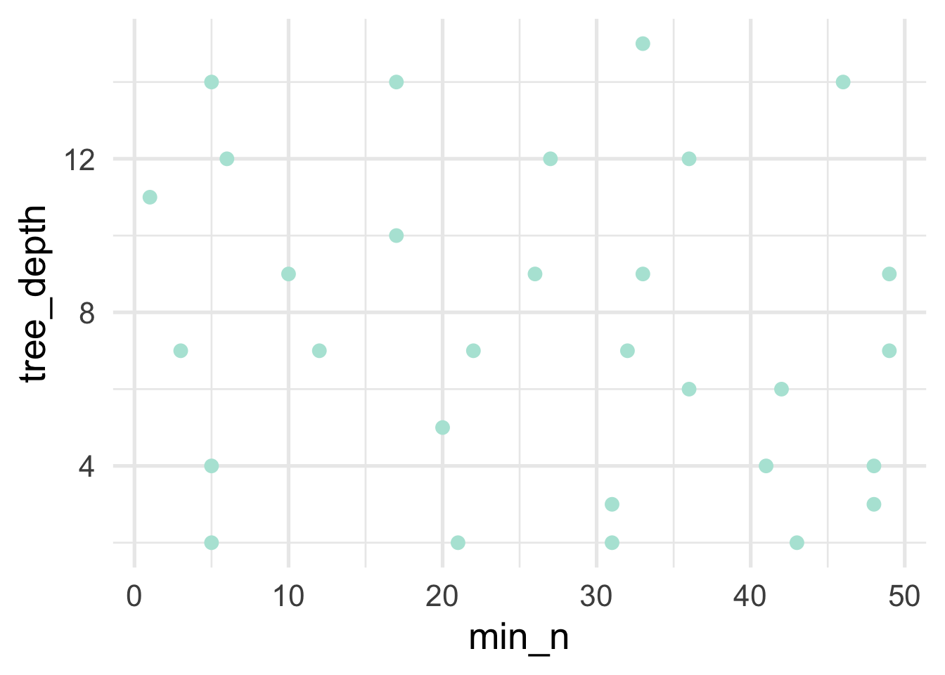
Looks pretty good! At least as a starting point. But we’ll want to look at the trends for each of these hyperparatmers after tuning to see if we need to further refine them.
Going forward from here with just the {tidymodels} implementation, we’ll set the learning rate at 0.05 and set each of the tree depth parameters to tune.
We’ll then fit the model (using high performance computing) for each of the combinations in our hyperparamter space-filling design using tune_grid().
Let’s evaluate the trends of each of the hyperparameters
collect_metrics(tune_treedepth_tm) %>%
  filter(.metric == "rmse") %>%
  pivot_longer(c("min_n", "tree_depth")) %>%
  ggplot(aes(value, mean)) +
  geom_line() +
  geom_point() +
  facet_wrap(~name, scales = "free_x")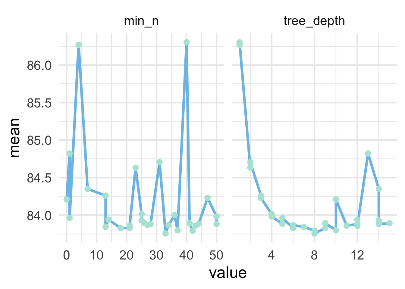
And we can see that the optimal value for min_n is a little bit less clear than for tree_depth. The former looks to be somewhere in the range of 12-25, but a few of the higher values (e.g., 33-ish) look pretty good as well. For the latter, it seems pretty clear that a tree depth of about 8 is optimal. Note that this is a bit higher than typical. Let’s look at just the raw
## # A tibble: 30 x 8
##    min_n tree_depth .metric .estimator  mean     n std_err .config
##    <int>      <int> <chr>   <chr>      <dbl> <int>   <dbl> <fct>
##  1    33          8 rmse    standard    83.8    10   0.411 Model17
##  2    42          8 rmse    standard    83.8    10   0.409 Model10
##  3    37         10 rmse    standard    83.8    10   0.403 Model16
##  4    18          9 rmse    standard    83.8    10   0.392 Model13
##  5    21          6 rmse    standard    83.8    10   0.414 Model03
##  6    13          7 rmse    standard    83.8    10   0.419 Model24
##  7    21         12 rmse    standard    83.9    10   0.397 Model14
##  8    43         11 rmse    standard    83.9    10   0.381 Model07
##  9    34          6 rmse    standard    83.9    10   0.404 Model25
## 10    27          6 rmse    standard    83.9    10   0.420 Model30
## # … with 20 more rows
And as we can see there are actually multiple combinations of our two hyperparameters that lead to essentially equivalentRMSE values. The variability (estimated by the standard error) is fairly consistent as well, although it is a bit lower for a few models. This is fairly common for boosted tree models and, really, any model with multiple hyperparameters - various combinations of the hyperparameters lead to similar results. Just to be certain this is really what we want, we could use a regular grid to search over min_n values from, say, 12 to 25 and 30 to 35 while tuning the tree depth over a smaller range, perhaps 6 to 9. For now, however, we’ll just move forward with our best combination from the grid search we’ve conducted. Let’s first update our model with the best hyperparameter combination we found. We’ll then proceed with model tuning to see if we can additional gains by limiting the depth of the tree by the change in the cost function (i.e, tuning the loss reduction).
mod <- mod %>%
  finalize_model(
    select_best(tune_treedepth_tm, metric = "rmse")
  ) %>%
  set_args(loss_reduction = tune())

mod
## Boosted Tree Model Specification (regression)
##
## Main Arguments:
## trees = 5000
## min_n = 33
## tree_depth = 8
## learn_rate = 0.05
## loss_reduction = tune()
## stop_iter = 20
##
## Engine-Specific Arguments:
## nthread = 16
## validation = 0.2
##
## Computational engine: xgboostLet’s search 15 different values of loss reduction, searching over the default recommended range provided to use by the dials::loss_reduction function
##  [1] 1.000000e-04 2.553541e-04 6.520572e-04 1.665055e-03 4.251786e-03
##  [6] 1.085711e-02 2.772408e-02 7.079458e-02 1.807769e-01 4.616212e-01
## [11] 1.178769e+00 3.010034e+00 7.686246e+00 1.962715e+01 5.011872e+01
Note that I have changed the default range here (after applying a log10 transformation) so there aren’t quite so many values down close to zero, and there are a few more that are in the upper range.
Let’s tune the model
And evaluate the how the loss reduction related to the RMSE:
## # A tibble: 15 x 7
##    loss_reduction .metric .estimator  mean     n std_err .config
##             <dbl> <chr>   <chr>      <dbl> <int>   <dbl> <fct>
##  1       0.0109   rmse    standard    83.7    10   0.401 Model06
##  2       0.00425  rmse    standard    83.7    10   0.404 Model05
##  3       3.01     rmse    standard    83.8    10   0.399 Model12
##  4       0.000652 rmse    standard    83.8    10   0.402 Model03
##  5       7.69     rmse    standard    83.8    10   0.396 Model13
##  6       0.000255 rmse    standard    83.8    10   0.378 Model02
##  7       0.0277   rmse    standard    83.8    10   0.406 Model07
##  8      50.1      rmse    standard    83.8    10   0.397 Model15
##  9       0.181    rmse    standard    83.8    10   0.380 Model09
## 10       0.0708   rmse    standard    83.8    10   0.409 Model08
## 11      19.6      rmse    standard    83.8    10   0.410 Model14
## 12       0.00167  rmse    standard    83.8    10   0.378 Model04
## 13       0.0001   rmse    standard    83.8    10   0.405 Model01
## 14       0.462    rmse    standard    83.9    10   0.399 Model10
## 15       1.18     rmse    standard    83.9    10   0.426 Model11
Our best model above is slightly better than our previous best, and the standard error (variance in the means across folds) is essentially unchanged. Let’s just look at these values quickly and make sure we don’t see any trends that would warrant additional tuning. Note that I’ve put a log 10 transformation on the x axis because that was the transformer that was used when creating the hyperparemeters, so that will allow us to view the hyperparameters with equal intervals.
collect_metrics(tune_lossred_tm) %>%
  filter(.metric == "rmse") %>%
  ggplot(aes(loss_reduction, mean)) +
  geom_line() +
  geom_point() +
  scale_x_log10()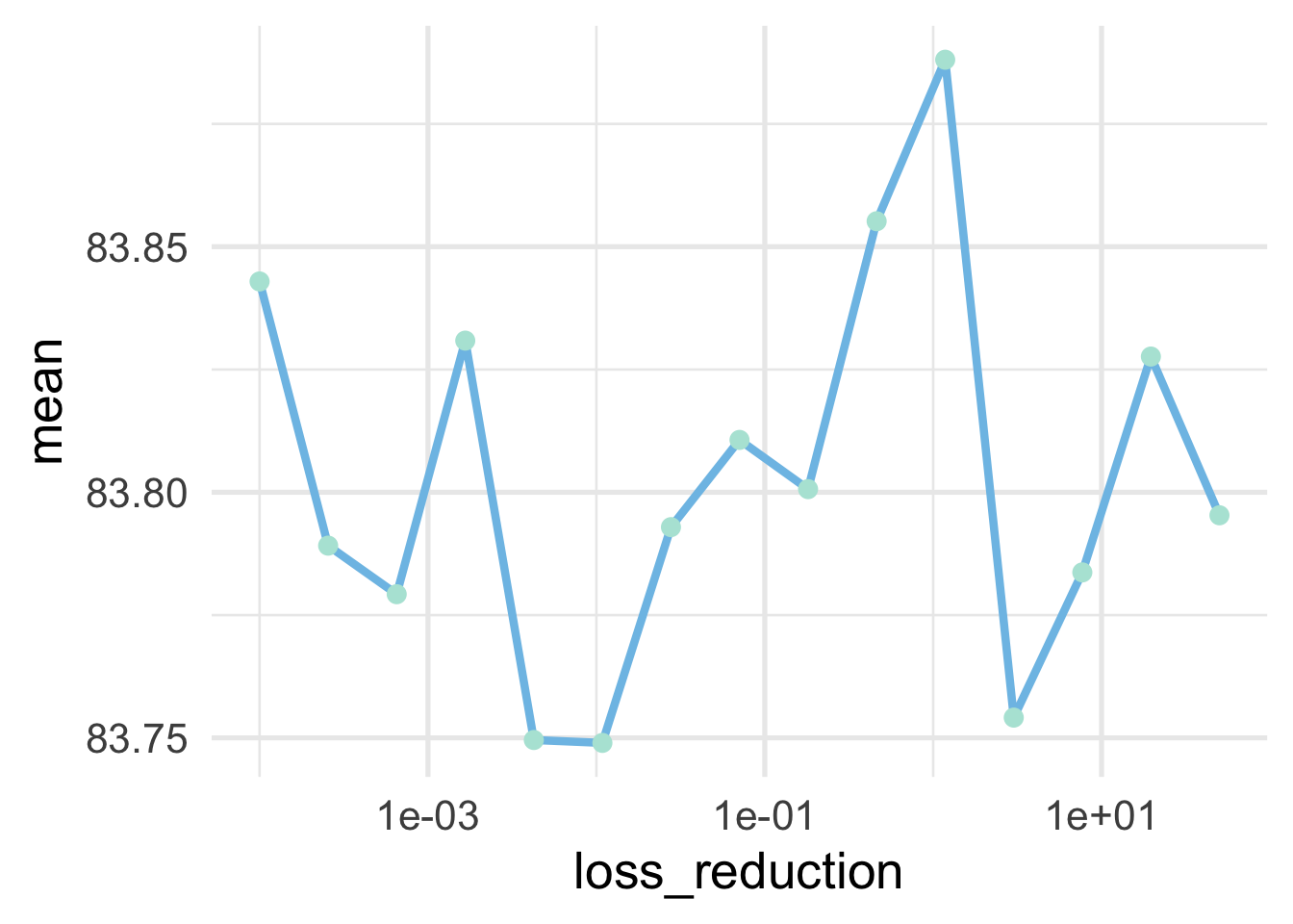
We don’t see much of a trend, and it’s important to note that the range of the y-axis is severely restricted (meaning all models are pretty comparable), but the two best values are on the lower end of the scale.
Let’s move forward with these, and tune the stochastic components. We’ll start by randomly sampling a proportion of rows and columns to sample for each tree (as opposed to each each split, as we do with random forests). We will again setup a grid for these parameters. To do this most efficiently, we’ll first bake our data so we can efficiently determine the number of rows and columns in our data. We will also use the dials::finalize() function to help us determine the range of reasonable values. This is because functions like dials::mtry() have a lower bound range of 1 (one column at a time) and an upper value that is unknown and depends on the number of columns in the data.
baked <- rec %>%
  prep() %>%
  bake(train) %>%
  select(-contains("id"), -ncessch)

cols_range <- finalize(mtry(), baked)
cols_range
## # Randomly Selected Predictors (quantitative)
## Range: [1, 62]For the sample_size argument {parsnip} expects (rather confusingly) a proportion of rows to be exposed to the fitting algorithm for each tree, rather than a number (i.e., at least as of thise writing, you will get an error if you used dials::sample_size() to determine the number of rows). We will therefore use sample_prop() and keep the default range from 10% to 100% of the rows.
Let’s again use a space-filling design to specify our grid, evaluating 30 different combinations of these hyperparameters.
## # A tibble: 30 x 2
##     mtry sample_size
##    <int>       <dbl>
##  1    60       0.350
##  2     4       0.221
##  3    59       0.655
##  4    53       0.361
##  5    61       0.762
##  6    56       0.204
##  7    43       0.171
##  8    35       0.167
##  9    19       0.827
## 10     4       0.656
## # … with 20 more rows
And finally, we can update our previous model with the best loss reduction, setting the stochastic parameters to tune. We then tune over our grid with tune_grid().
mod <- mod %>%
  finalize_model(select_best(tune_lossred_tm, metric = "rmse")) %>%
  set_args(sample_size = tune(),
           mtry = tune())
mod
## Boosted Tree Model Specification (regression)
##
## Main Arguments:
## mtry = tune()
## trees = 5000
## min_n = 33
## tree_depth = 8
## learn_rate = 0.05
## loss_reduction = 0.010857111194022
## sample_size = tune()
## stop_iter = 20
##
## Engine-Specific Arguments:
## nthread = 16
## validation = 0.2
##
## Computational engine: xgbooststoch_mets <- collect_metrics(tune_stoch_tm) %>%
filter(.metric == "rmse") %>%
arrange(mean)
stoch_mets## # A tibble: 30 x 8
## mtry sample_size .metric .estimator mean n std_err .config
## <int> <dbl> <chr> <chr> <dbl> <int> <dbl> <fct>
## 1 32 0.921 rmse standard 83.6 10 0.391 Model12
## 2 51 0.984 rmse standard 83.7 10 0.391 Model05
## 3 27 0.822 rmse standard 83.7 10 0.400 Model14
## 4 62 0.962 rmse standard 83.7 10 0.395 Model27
## 5 18 0.810 rmse standard 83.7 10 0.398 Model11
## 6 36 0.809 rmse standard 83.7 10 0.383 Model02
## 7 32 0.637 rmse standard 83.7 10 0.393 Model29
## 8 54 0.747 rmse standard 83.8 10 0.411 Model07
## 9 10 0.954 rmse standard 83.8 10 0.407 Model08
## 10 47 0.693 rmse standard 83.8 10 0.392 Model16
## # … with 20 more rowsAnd once again our best model is very marginally better over our previous best. Let’s see if there are any trends in these hyperparameters.
stoch_mets %>%
  pivot_longer(c(mtry, sample_size)) %>%
  ggplot(aes(value, mean)) +
  geom_line() +
  geom_point() +
  facet_wrap(~name, scales = "free_x")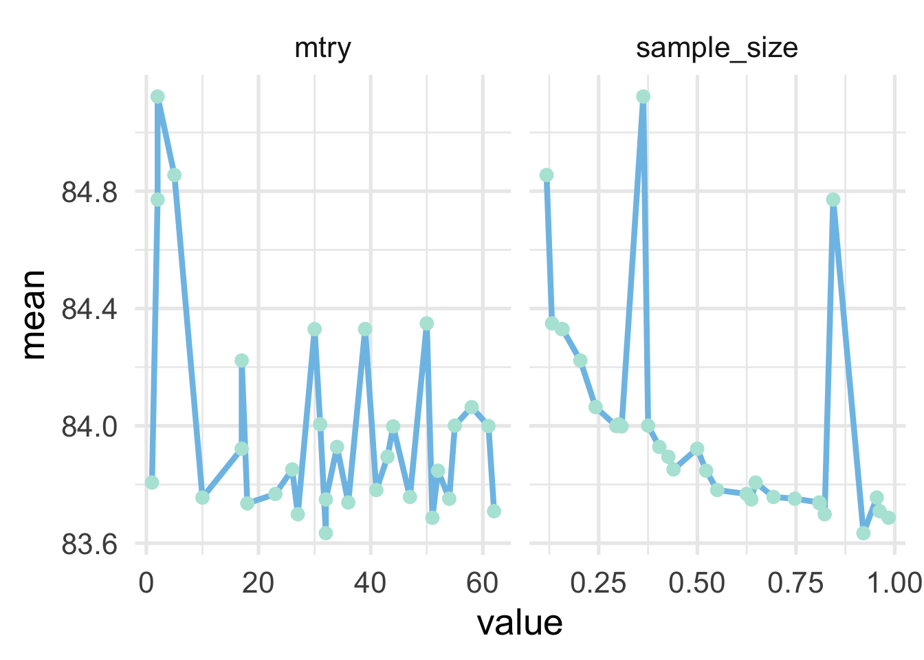
There doesn’t appear to be much of a trend in mtry, although values abouve about 10 seem to be preferred. For sample_size, there is a fairly clear trend downward as the proportion goes up, but the best is before we reach all the data. We might want to retune here with a more limited range on sample size somewhere between the 0.9 to 1.0 range, but we’ll leave here for now.
The final step for tuning this model would be to set the stochastic components and re-tune the learning rate to see if we could improve performance further. Given where we’ve been, and the progress we’ve made, our model is unlikely to have substantial performance improvements from here, but we might be able to make some marginal gains. In this case, we also didn’t have much evidence that our model was overfitting. If we did, we could try to tune on hyperparameters that are not currently implemented in parsnip::boost_tree(), like L1 and L2 regularizers, by just passing these arguments direction to the {xgboost} function through set_args(). We just need to use the name of the parameter in {xgboost}. For example
mod <- mod %>%
  finalize_model(select_best(tune_stoch_tm, metric = "rmse")) %>%
  set_args(
    alpha = tune(), # L1
    lambda = tune() # L2
  )
Then we set a grid. I’ve used a space filling design below and the method is a bit hacky because grid_max_entropy won’t let us have two penalty() values, and it also won’t (currently) let us have two named values. So we just create it with different names and then manually rename the columns.
penalized_grid <- grid_max_entropy(penalty(), lambda = penalty(), size = 15)
names(penalized_grid)[1] <- "alpha"
penalized_grid
## # A tibble: 15 x 2
## alpha lambda
## <dbl> <dbl>
## 1 3.15e-10 1.49e-10
## 2 5.67e- 4 3.60e- 3
## 3 4.66e- 3 1.28e- 9
## 4 8.06e- 3 9.35e- 6
## 5 6.09e- 6 4.85e- 2
## 6 5.06e- 8 3.41e- 8
## 7 2.56e- 2 6.72e- 1
## 8 1.48e- 8 7.90e- 1
## 9 1.95e- 5 3.30e- 6
## 10 7.86e- 8 1.25e- 4
## 11 1.54e- 1 2.62e- 4
## 12 3.21e-10 1.05e- 5
## 13 9.16e- 1 1.15e- 6
## 14 1.72e- 5 2.17e-10
## 15 6.71e-10 1.56e- 2And then we can tune. Note that we are not actually fitting this model here, but rather we are illustrating how you can tune hyperparameters with {tidymodels} that are not yet implemented in the given {parsnip} model.
Note that if we wanted to try a different booster, such as DART (which uses dropout), we would need to use {xgboost} directly.
35.3.2 Wrapping up
Gradient boosted trees provide a powerful framework for constructing highly performant models. They differ from other tree-based ensemble models by building the trees sequentially, with each new tree fit to the errors of the previous. The learning is guided by gradient descent, an algorithm that finds the optimal direction the model needs to move in to minimize the objective function. The rate at which we move in that direction, is called the learning rate.
Gradient boosted trees, particularly when implemented with {xgboost} have a large number of hyperparameters - many more than we’ve seen in previous models. This means that multiple combinations of these hyperparameters may lead to similarly performing models. It can also become overwhelming if you are searching for any combination that even marginally improves performance, as with online machine learning competition platforms like Kaggle. In most social science problems, however, the practical difference in a model that has an RMSE value of (in our example) 83.8 versus, say, 83.6 is unlikely to be a game changer. If it is, then you should likely go through several cycles of hyperparameter tuning to try to identify the optimal hyperparameter combination. But if it’s not, we suggest proceeding in the method shown here, using early stopping to control the number of trees, tuning the learning rate, then the tree-specific hyperparemters, and then the stochastic components. After conducting those steps, you should re-evaluate the learning rate and, in particular, see if a reduced learning rate will increase model performance. From there, we would likely move on and call our model complete. Knowing when to push for more model performance, and when to abandon you efforts and live with what you have, is part of the “art” to building predictive models, and this intuition builds both with experience and with your own knowledge of the data.