34 Bagging and Random Forests

In the last chapter, we talked about how decision trees are highly flexible, but are often not the most performant model on their own because they can easily overfit, leading to poor generalizability to new/unseen data. One way to avoid this problem is to build an ensemble of trees from random bootstrap samples of the data, and aggregate the predictions across the entire ensemble. This is a general approach known as bagging, or bootstrap aggregation, which can be applied to any modeling framework, but generally will only provide large gains in improvement if, like decision trees, the model has high variability.

Bagging

A general process to improve the performance of highly variable models, regularly applied to decision trees.

Create $b$ bootstrap resamples of the original data
Fit the model (base learner) to each $b$ resample
Aggregate predictions across all models

For regression problems, the final prediction is the average of all model predictions
For classification problems, either (a) average model classification probabilities or (b) take the mode of model classifications.

Benefits: Leads to more stable model predictions (reduces model variability)

As mentioned previously, bagging does not tend to help much (and increases computational burdens) when the model already has low variance. Models like linear regression will generally not change much in their model predictions when using bagging. For example, for a very small sample, bagging may help a linear model, but as the sample size grows, the predictions will be nearly identical while increasing computational complexity. Decision trees, however, can be highly variable. Bagging can help reduce the variance of these models and lead to more stable model predictions.

How many bags?

Put differently, how many bootstrap resamples?

There is no hard and fast rule. The important thing is to have enough bags to reach a stable model.

Noisier data will require more bags. Data with strongly predictive features will require fewer bags.

Start with somewhere between between 50-500 bags depending on how variable you think your data are, evaluate the learning curve, and then adjust up or down from there accordingly.

There is no rule for the number of “bags”, or bootstrap resamples, that one should use to create a stable model. Further, the number of bags just needs to be sufficiently high that the model becomes stable—after stability is achieved, additional bags will not help model performance. In other words, there is no upper bound for the number of bags (the only burden is computational), but it is critical that there are enough bags to create a stable model. Datasets with highly predictive features will generally need fewer bags to reach stability.

34.0.1 Bagging “by hand”

To understand bagging we first have to be clear about what bootstrap resampling implies. When we take bootstrap resamples from our dataset, we sample $n$ rows of our dataset with replacement, where $n$ represents the total number of rows in our data. For example, suppose we had a dataset that had the first five letters of the alphabet, each with an associated score.

lets <- data.frame(letters = c("a", "b", "c", "d", "e"),
                   score = c(5, 7, 2, 4, 9))
lets

##   letters score
## 1       a     5
## 2       b     7
## 3       c     2
## 4       d     4
## 5       e     9

Bootstrap resampling would imply sampling five rows from the above dataset with replacement. This means some rows may be represented multiple times, and others not at all. Let’s do this and see what the first three datasets look like.

# set seed for reproducibility
set.seed(42)

# specify the number of bootstrap resamples
b <- 3
resamples <- replicate(b, 
                       lets[sample(1:5, 5, replace = TRUE), ],
                       simplify = FALSE)
resamples

## [[1]]
##     letters score
## 1         a     5
## 5         e     9
## 1.1       a     5
## 1.2       a     5
## 2         b     7
## 
## [[2]]
##     letters score
## 4         d     4
## 2         b     7
## 2.1       b     7
## 1         a     5
## 4.1       d     4
## 
## [[3]]
##     letters score
## 1         a     5
## 5         e     9
## 4         d     4
## 2         b     7
## 2.1       b     7

Notice that in the first bootstrap resample, a is represented three times, b once, c and d not at all, and e once. Similar patterns, with different distributional frequencies, are represented in the second and third datasets.

Why is this useful? It turns out that if we do this enough times, we develop a sampling distribution. Fitting the model to all of these different samples then gives us an idea of the variability of the model, which we can reduce by averaging across all samples. Bootstrap resampling is useful in all sorts of different ways in statistics. In the above, our observed mean across the letters is 5.4. We can compute the standard error of this mean analytically by $\sigma/\sqrt{n}$, or sd(lets$score)/sqrt(5), which is equal to 1.2083046. We can also approximate this same standard error by computing the mean of many bootstrap resamples, and estimating the standard deviation among these means. For example

library(tidyverse)

b <- 5000
resamples <- replicate(b, 
                       lets[sample(1:5, 5, replace = TRUE), ],
                       simplify = FALSE)
means <- map_dbl(resamples, ~mean(.x$score))
sd(means)

## [1] 1.108987

In this case, the difference between the analytic standard error and the bootstrap estimate is greater than typical because the sample size is so small.

The process of bagging is essentially equivalent to the above, except instead of computing the mean with each bootstrap resample, we fit a full model. We then compute the predictions from all of these models and either average the resulting predictions, or take the mode of the classifications.

34.1 Bagged trees

The {baguette} package, part of the {tidymodels} metapackage, provides an interface for bagging in R. It is not part of the core set of packages, implying it is installed with {tidymodels} but not loaded. You must load {baguette} outside of your call to {tidymodels} (i.e., similar to the {lubridate} package in the {tidyverse}).

Recall our best model when fitting a decision tree in the previous chapter had an average AUC across folds of $0.825$. This included a very low cost complexity parameter of $0.0000000001$ and a minimum $n$ for our terminal nodes of 35. Can we improve performance from this model when using bagging? Let’s try!

First, we need to load the data, create a split training/test set, pull the training data, and create a $k$-fold cross-validation dataset. Some of the models we’ll be working with cannot handle missingness on the outcome, so we’ll remove these rows upon reading the data into R.

library(tidyverse)
library(tidymodels)
library(sds)

k_train <- get_data("ds-bowl-2019")

splt <- initial_split(k_train)
train <- training(splt)
cv <- vfold_cv(train)

Next, we’ll specify a basic recipe that just specifies the model formula.

rec <- recipe(accuracy_group ~ ., data = train)

And now we’re ready to specify our model. This is pretty much the same as before, except now we are going to load the {baguette} package in addition to {tidymodels} and use bag_tree() instead of decision_tree(). Additionally, we’ll specify a times argument when we set the engine. Let’s start by fitting a model to 50 bootstrap resamples and aggregating the results across all 50 trees. The rest is the same as before.

Let’s start by by building a very deep tree, with no pruning and a minimum sample size for the terminal nodes of 2. First we’ll set the model.

library(baguette)
library(tictoc)

bt_mod <- bag_tree() %>% 
  set_engine("rpart", times = 50) %>%  #50 bootstrap resamples or bags
  set_mode("classification") %>% 
  set_args(cost_complexity = 0,
           min_n = 2)

and then we’ll fit it to the $k$ folds.

The code below took about 13.5 minutes to fit on a local computer.

bt_fit1 <- fit_resamples(bt_mod,
                       preprocessor = rec,
                       resamples = cv)

Then we can look at the performance of the model.

collect_metrics(bt_fit1)

## # A tibble: 2 x 5
##   .metric  .estimator  mean     n std_err
##   <chr>    <chr>      <dbl> <int>   <dbl>
## 1 accuracy multiclass 0.500    10 0.00222
## 2 roc_auc  hand_till  0.706    10 0.00182

That’s a pretty decent gain! But how do we know that 50 bags is enough? We can create a learning curve by fitting our model to many different bootstrap resample values, and evaluate the objective function for each of these values. To do that, let’s write a function that specifies a model with any bootstrap value, $b$, fits the model, and then extracts the AUC.

Remember, we only need to find the value where our objective function stablizes. Adding additional bootstrap resamples won’t hurt in terms of model performance, but it will cost us in terms of computational time. So we want to use a value of $b$ that is around the lowest possible value once stability has been reached (so we don’t waste computational time).

When we fit the model above, we used fit_resamples() using 10-fold cross validation. This time, we only want to get a rough estimate of model stability. So, to save on computation time, let’s create a small cv object with just two folds, then use this to fit all the $b$ candidate models.

# specify a small cv
small_cv <- vfold_cv(train, v = 2)

pull_auc <- function(b) {
  # specify model
  mod <- bag_tree() %>% 
    set_mode("classification") %>% 
    set_args(cost_complexity = 0, min_n = 2) %>% 
    set_engine("rpart", times = b)
  
  # fit model to full training dataset
  m <- fit_resamples(mod, rec, small_cv)
  
  # extract the AUC & add the $b$ value
  auc <- show_best(m, "roc_auc") 
  auc$b <- b
  
  # return the AUC data frame
  auc
}

Now we just need to specify a vector of candidate bags, $b$, and loop our function through this vector. We’ll look at values between $5$ and $305$ by increments of 25. Note that we have used parallel processing here again to help speed things along via the {future} package. However, this is still a highly computationally intensive operation. We’ll talk about more efficient ways to do this in the next section.

The code below took approximately 3 hours and 45 minutes to run on a local computer.

# specify candidate b models
b <- seq(5, 305, 25)

# Fit models
library(future)
plan(multisession)
tic()
aucs <- map_df(b, pull_auc)
toc()

plan(sequential)

Let’s plot these samples now to see when we reach stability. Note

ggplot(aucs, aes(b, mean)) +
  geom_line() +
  geom_point()

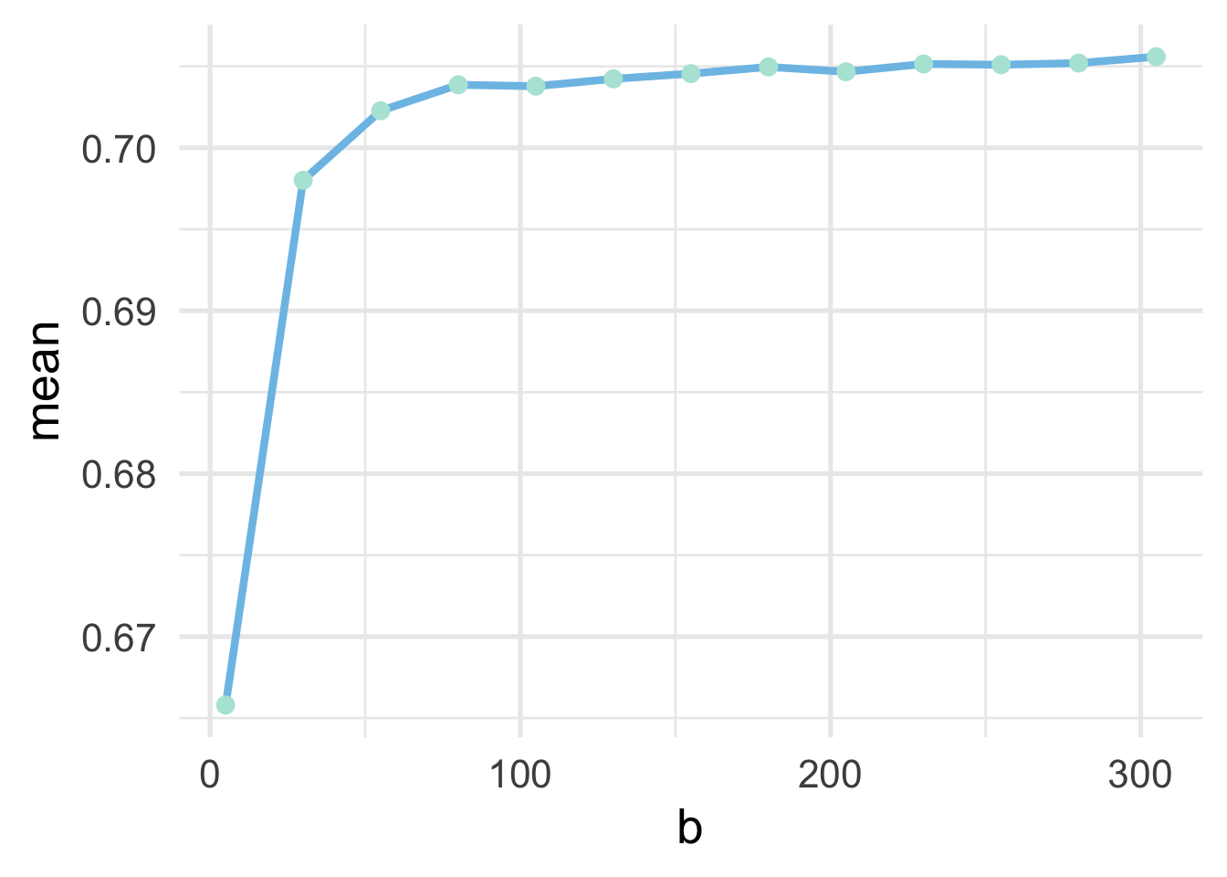
And it looks like after about 150 bags the model becomes stable.

Moving forward, we could proceed with model tuning just as we did before, using $k$-fold cross validation, and using a bagged tree model with $b = 150$. However, as the process above illustrates, this can be a highly computationally intensive process. We would need to fit decision trees to each of 200 bootstrap resamples, for each of the $k$ folds for every hyperparameter we evaluated. In the Decision Trees chapter, we evaluated 50 hyperparamters in our initial model tuning (10 for cost complexity and 5 for the minimum $n$ size for a terminal node). Assuming 10-fold cross-validation, this would result in $50 \times 10 \times 150 = 75000$ decision trees! That’s going to take a long time. Luckily, there are alternative options.

34.1.1 Working with out-of-bag samples

Recall from our chapter on cross-validation procedures that there are multiple approaches to cross-validation, including bootstrap resampling. When using boostrap resampling for cross-validation, we fit a candidate model on the boostrapped data, and evaluate it against the cases that were not included in the bootstrap. For example, if our data looked like this:

lets

##   letters score
## 1       a     5
## 2       b     7
## 3       c     2
## 4       d     4
## 5       e     9

and our bootstrap resample looked like this

resamples[[1]]

##     letters score
## 3         c     2
## 1         a     5
## 1.1       a     5
## 3.1       c     2
## 4         d     4

Then we would fit our model to letters a, b, and e, and evaluate our model by making predictions for letters c and d.

If you’re using bagging to develop a model, you already have bootstrap resamples. The out-of-bag (OOB) samples are then “free”, computationally. If your sample size is reasonably large ($n > 1000$) the OOB estimates of model performance will be similar to those obtained from $k$-fold CV, but take only a fraction of the time.

Unfortunately, as of the time of this writing, there is no way to easily access the OOB samples with {baguette}. Luckily, we can fit the model in a slightly different way, using the {ranger} package, and this will allow us to access the OOB samples.

In what follows, we’ll use {ranger} within a {tidymodels} framework to fit and tune a bagged tree model using the OOB samples. The {ranger} package is designed to fit random forests, which we’ll talk about next. Bagged trees, however, are just a special case of random forests where there is no sampling of columns when each tree is built (more on this soon). To fit a bagged tree with {ranger}, we just have to set the mtry argument equal to the number of predictors in our data frame.

Let’s start by re-fitting our bt_mod1 model with {ranger}, using the OOB samples for our model performance. To do this, we’re going to use the fit() function, instead of fit_resamples() (because we’re only going to be fitting the model once). We will therefore need to prep() and bake() our recipe to get our processed training data.

processed_train <- rec %>% 
  prep() %>% 
  bake(new_data = NULL)

processed_train

## # A tibble: 65,047 x 6
##    event_count event_code game_time title               world     accuracy_group
##          <dbl>      <dbl>     <dbl> <fct>               <fct>     <ord>         
##  1          43       3020     25887 Bird Measurer (Ass… TREETOPC… 0             
##  2          28       3121     19263 Cauldron Filler (A… MAGMAPEAK 2             
##  3          76       4020     76372 Chest Sorter (Asse… CRYSTALC… 1             
##  4           1       2000         0 Bird Measurer (Ass… TREETOPC… 2             
##  5          39       4025     44240 Chest Sorter (Asse… CRYSTALC… 0             
##  6          21       4020     14421 Cart Balancer (Ass… CRYSTALC… 3             
##  7          30       3110     21045 Cart Balancer (Ass… CRYSTALC… 3             
##  8          40       3121     28769 Cart Balancer (Ass… CRYSTALC… 3             
##  9           2       2020        51 Cart Balancer (Ass… CRYSTALC… 3             
## 10          15       3021      8658 Mushroom Sorter (A… TREETOPC… 3             
## # … with 65,037 more rows

Next, it’s helpful to determine the number of predictors we have with code. In this case, it’s fairly straightforward, but occassionally things like dummy-coding can lead to many new columns, and zero or near-zero variance filters may remove columns, so it’s worth double-checking our assumptions.

ncol(processed_train) - 1

## [1] 5

Note that we subtract one from the number of columns because we are only counting predictors (not the outcome).

Next, we specify the model. Notice we use rand_forest() here for our model, even though we’re actually fitting a bagged tree, and we set mtry = 5. The number of bags is set by the number of trees. Note that, while we found a higher value is likely better, we’ve set the number of trees below to be 50 so the model is comparable to bt_mod. There is no pruning hyperparameter with {ranger}, but we can set the min_n to 2 as we had it before. The below code includes one additional argument that is passed directly to {ranger}, probability = FALSE, which will make the predictions from the model be the actual classes, instead of the probabilities in each class.

bt_mod2 <- rand_forest() %>% 
  set_engine("ranger") %>% 
  set_mode("classification") %>% 
  set_args(mtry = 5, # Specify number of predictors
           trees = 50, # Number of bags
           min_n = 2,
           probability = FALSE)

Now we just fit the model to our processed data. We’re using the {tictoc} package to time the results.

library(tictoc)
tic()
bt_fit2 <- fit(bt_mod2,
               accuracy_group ~ .,
               processed_train)
toc(log = TRUE) # `log = TRUE` so I can refer to this timing later

## 16.797 sec elapsed

As you can see, we have substantially cut the fitting time down because we’ve only fit the model once, and it now fits in 16.8 seconds! But do we get the same estimates for our metrics if we use the OOB samples? Let’s look at the model object

bt_fit2

## parsnip model object
## 
## Fit time:  15.6s 
## Ranger result
## 
## Call:
##  ranger::ranger(x = maybe_data_frame(x), y = y, mtry = min_cols(~5,      x), num.trees = ~50, min.node.size = min_rows(~2, x), probability = ~FALSE,      num.threads = 1, verbose = FALSE, seed = sample.int(10^5,          1)) 
## 
## Type:                             Classification 
## Number of trees:                  50 
## Sample size:                      65047 
## Number of independent variables:  5 
## Mtry:                             5 
## Target node size:                 2 
## Variable importance mode:         none 
## Splitrule:                        gini 
## OOB prediction error:             50.32 %

This says that our OOB prediction error is 50.32. Our accuracy is one minus this value, or 49.68. Using $k$-fold cross validation we estimated our accuracy at 50.03. So we’re getting essentially the exact same results, but using the OOB samples much faster!

What if we want other metrics? We can access the OOB predictions from our model using bt_fit2$fit$predictions. We can then use these predictions to calculate OOB metrics via the {yardstick} package, which is used internally for functions like collect_metrics(). For example, assume we wanted to estimate the OOB AUC. In this case, we would need to re-estimate our model to get the predicted probabilites for each class.

bt_mod3 <- rand_forest() %>% 
  set_engine("ranger") %>% 
  set_mode("classification") %>% 
  set_args(mtry = 5,
           trees = 50,
           min_n = 2,
           probability = TRUE) # this is the default

bt_fit3 <- fit(bt_mod3,
               accuracy_group ~ .,
               processed_train)

Now we just pull the OOB predicted probabilities for each class, and add in the observed class.

preds <- bt_fit3$fit$predictions %>% 
  as_tibble() %>% 
  mutate(observed = processed_train$accuracy_group)

preds

## # A tibble: 65,047 x 5
##       `0`    `1`    `2`   `3` observed
##     <dbl>  <dbl>  <dbl> <dbl> <ord>   
##  1 0.912  0.0882 0      0     0       
##  2 0      0.05   0.1    0.85  2       
##  3 0      1      0      0     1       
##  4 0.316  0.284  0.127  0.273 2       
##  5 1      0      0      0     0       
##  6 0.0217 0.304  0.0435 0.630 3       
##  7 0.429  0      0.452  0.119 3       
##  8 0.0667 0.133  0.533  0.267 3       
##  9 0.321  0      0      0.679 3       
## 10 0.529  0.235  0      0.235 3       
## # … with 65,037 more rows

And now we can use this data frame to estimate our AUC, using yardstick::roc_auc().

roc_auc(data = preds, truth = observed, `0`:`3`)

## # A tibble: 1 x 3
##   .metric .estimator .estimate
##   <chr>   <chr>          <dbl>
## 1 roc_auc hand_till      0.699

How does this compare to our estimate with 10-fold CV?

collect_metrics(bt_fit1)

## # A tibble: 2 x 5
##   .metric  .estimator  mean     n std_err
##   <chr>    <chr>      <dbl> <int>   <dbl>
## 1 accuracy multiclass 0.500    10 0.00222
## 2 roc_auc  hand_till  0.706    10 0.00182

It’s very close and, again, took a fraction of the time.

34.1.2 Tuning with OOB samples

If we want to conduct hyperparameter tuning with a bagged tree model, we have to do to a bit more work, but it’s not too terrible. Let’s train on minimum $n$ and set the number of trees to be large—say, 200.

Much like we did before, we’ll write a function that fits a model for any min_n value. We’ll optimize our model by trying to maximize AUC, so we’ll have our function return the OOB AUC estimate, along with the $n$ size that was used for the terminal nodes.

tune_min_n <- function(n) {
  mod <- rand_forest() %>% 
    set_mode("classification") %>% 
    set_engine("ranger") %>% 
    set_args(mtry = 5,
             min_n = n,
             trees = 200)
  
  # fit model to full training dataset
  m <- fit(mod, accuracy_group ~ ., processed_train)
  
  # create probabilities dataset
  pred_frame <- m$fit$predictions %>% 
    as_tibble() %>% 
    mutate(observed = processed_train$accuracy_group)
  
  # calculate auc
  auc <- roc_auc(pred_frame, observed, `0`:`3`) %>% 
    pull(.estimate) # pull just the estimate
  
  # return as a tibble
  tibble(auc = auc, min_n = n)
}

Now we can loop through a bunch of $n$ sizes for the terminal nodes and see which provides us the best OOB AUC values for a bagged tree with 200 bags. We’ll use map_df() so the results are bound into a single data frame. Let’s search through values from 2 to 50 and see how the OOB AUC changes.

The code chunk below takes about 20 minutes to run on a local computer.

min_n_aucs <- map_df(2:50, tune_min_n)

Let’s plot the learning curve.

ggplot(min_n_aucs, aes(min_n, auc)) +
  geom_line(color = "gray40") +
  geom_smooth(se = FALSE)

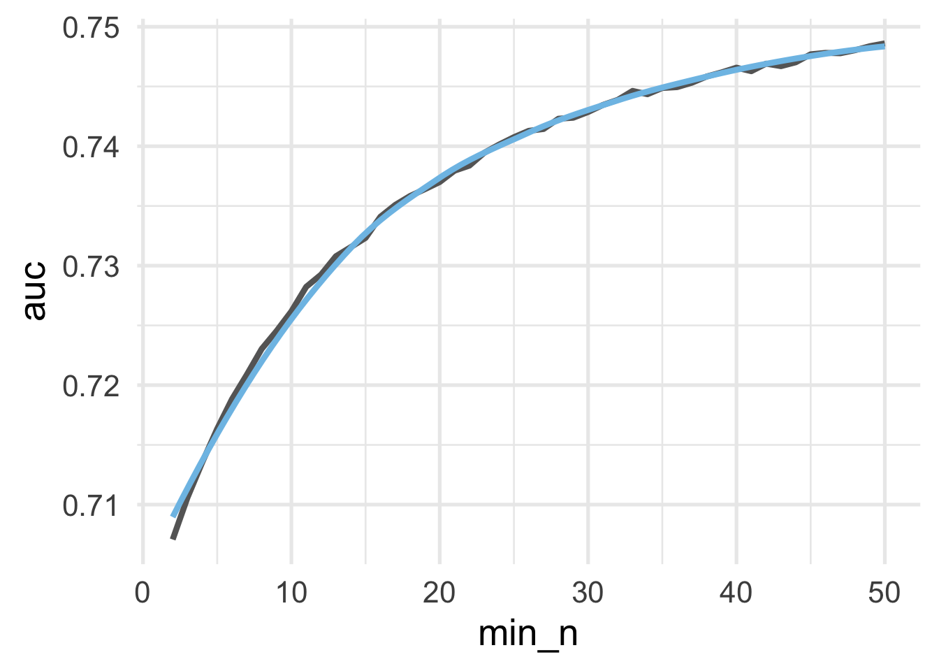
Because we are trying to maximize AUC, the ideal value appears to be somewhere around 15. Let’s extract the maximum AUC $n$.

max_auc <- min_n_aucs %>% 
  filter(auc == max(auc))

max_auc

## # A tibble: 1 x 2
##     auc min_n
##   <dbl> <int>
## 1 0.749    50

And now we’re likely ready to finalize our model. Let’s evaluate it against our test set.

final_mod <- rand_forest() %>% 
    set_mode("classification") %>% 
    set_engine("ranger") %>% 
    set_args(mtry = 5,
             min_n = 13,
             trees = 200)

final_fit <- last_fit(final_mod, rec, splt)
final_fit$.metrics

## [[1]]
## # A tibble: 2 x 3
##   .metric  .estimator .estimate
##   <chr>    <chr>          <dbl>
## 1 accuracy multiclass     0.546
## 2 roc_auc  hand_till      0.738

And our final AUC estimate on our test set is essentially equivalent to what we found during training using our OOB samples

34.2 Random Forests

One potential problem with bagged trees is that the predictions across trees often correlate strongly. This is because, even if a new bootstrap sample is used to create the tree, all of the features are used in every tree. Thus, if a given feature is strongly predictive of the outcome, it is likely to be used as the root node in nearly every tree. Because decision trees are built recursively, with optimal splits only determined after previous splits have already been determined, this means that we may be missing out on potential predictive accuracy by not allowing other features to “start” the tree (be the root node). This does not mean that bagging is not useful. As we just saw, we were able to have fairly substantial gains in model performance using bagging when compared to what we observed with a single tree. Yet, if we could decorrelate the trees, we might be able to improve performance even more.

Random forests extend bagged trees by introducing a stochastic component to the features. Specifically, rather than building each tree with all of the features, each tree is built using a random sample of features at each split. The predictive performance of any individual tree is then unlikely to be as performant as a tree using all the features at each split, but the forest of trees (aggregate prediction) can regularly provide better predictions than any single tree.

Assume we have a feature with one very strong predictor and a few features that are moderately strong predictors. If we used bagging, the moderately strong predictors would likely be internal nodes for nearly every tree–meaning their importance would be conditional on the strong predictor. Yet, these variables might provide important information for specific samples on their own. If we remove the very strong predictor from the root node split, that tree will be built with one of the moderately strong predictors at the root node. The very strong predictor may then be selected in one of the internal nodes and, while this model may not be as predictive overall, it may result in better predictions for specific cases. If we average over all these diverse models, we can often get better predictions for the entire dataset.

In essence, a random forest is just a bagged tree with a stochastic component introduced to decorrelate the trees. This means each individual model is more different than a bagged tree. When we average across all the trees we reduce this variance and may be able to get overall improved performance when compared to a single tree or a bagged tree.

Random forests work like bagged trees, but include a random selection of features at each split. This helps decorrelate the trees and can help get at the unique features of the data.

Random forest models tend to provide very good “out of the box” model performance. Because bagged trees are just a special case of random forests, and the number of predictors to select for each tree is a hyperparameter that can be tuned, it’s generally worth starting with a random forest and only moving to a bagged tree if, for your specific situation, using all the predictors for each tree works better than using a sample.

34.2.1 Fitting random forests

In the previous section we used the rand_forest() function to fit bagged classification trees and obtain performance metrics on the OOB samples. We did this by setting mtry = p, where p is equal to the number of predictor variables. When fitting a random forest, we just change mtry to a smaller value, which represents the number of features to randomly select from at each split. Everything else is the same: trees represents the number of bags, or the number of trees in the forest, while min_n represents the minimum sample size for a terminal node (i.e., limiting the depth to which each tree is grown).

A good place to start is mtry = p/3 for regression problems and mtry = sqrt(p) for classification problems. Generally, higher values of mtry will work better when the data are fairly noisy and the predictors are not overly strong. Lower values of mtry will work better when there are a few very strong predictors.

Just like bagged trees, we need to have a sufficient number of trees that the performance estimate stabilizes. Including more trees will not hurt your model performance, but it will increase computation time. Generally, random forests will need more trees to stabilize than bagged trees, because each tree is “noisier” than those in a bagged tree. A good place to start is at about 1,000 trees, but if your learning curve suggests the model is still trending toward better performance (rather than stabilizing/flat lining) then you should add more trees. Note that the number of trees you need will also depend on other hyperparameters. Lower values of mtry and min_n will likely lead to needing a greater number of trees.

Because we’re using bagging in a random forest we can again choose whether to use $k$-fold cross validation or just evaluate performance based on the OOB samples. If we were in a situation where we wanted to be extra sure we had conducted the hyperparameter tuning correctly, we might start by building a model on the OOB metrics, then evaluate a small candidate of hyperparameters with $k$-fold CV to finalize them. In this case we will only use the OOB metrics to save on computation time.

34.2.1.1 A classification example

Let’s continue with our classification example, using the same training data and recipe we used in the previous section. As a reminder, the recipe looked like this:

rec <- recipe(accuracy_group ~ ., data = train)

And we prepared the data for analysis so it looked like this:

processed_train <- rec %>% 
  prep() %>% 
  bake(new_data = NULL)

processed_train

## # A tibble: 65,047 x 6
##    event_count event_code game_time title               world     accuracy_group
##          <dbl>      <dbl>     <dbl> <fct>               <fct>     <ord>         
##  1          43       3020     25887 Bird Measurer (Ass… TREETOPC… 0             
##  2          28       3121     19263 Cauldron Filler (A… MAGMAPEAK 2             
##  3          76       4020     76372 Chest Sorter (Asse… CRYSTALC… 1             
##  4           1       2000         0 Bird Measurer (Ass… TREETOPC… 2             
##  5          39       4025     44240 Chest Sorter (Asse… CRYSTALC… 0             
##  6          21       4020     14421 Cart Balancer (Ass… CRYSTALC… 3             
##  7          30       3110     21045 Cart Balancer (Ass… CRYSTALC… 3             
##  8          40       3121     28769 Cart Balancer (Ass… CRYSTALC… 3             
##  9           2       2020        51 Cart Balancer (Ass… CRYSTALC… 3             
## 10          15       3021      8658 Mushroom Sorter (A… TREETOPC… 3             
## # … with 65,037 more rows

We will again optimize on the model AUC. Recall that we had 5 predictor variables. Let’s start by fitting a random forest with 1,000 trees, randomly sampling two predictors at each split ($\sqrt{5}=2.24$). We’ll set min_n to 2 again so we are starting our modeling process by growing very deep trees

rf_mod1 <- rand_forest() %>% 
    set_mode("classification") %>% 
    set_engine("ranger") %>% 
    set_args(mtry = 2,
             min_n = 2,
             trees = 1000)
tic()
rf_fit1 <- fit(rf_mod1, 
               formula = accuracy_group ~ .,
               data = processed_train)
toc()

## 75.51 sec elapsed

Note that even with 1,000 trees, the model fits very quickly. What does our AUC look like for this model?

pred_frame <- rf_fit1$fit$predictions %>% 
  as_tibble() %>% 
  mutate(observed = processed_train$accuracy_group)

roc_auc(pred_frame, observed, `0`:`3`)

## # A tibble: 1 x 3
##   .metric .estimator .estimate
##   <chr>   <chr>          <dbl>
## 1 roc_auc hand_till      0.751

Looks pretty good! Note that this is quite similar to the best value we estimated using a bagged tree.

But did our model stabilize? Did we use enough trees? Let’s investigate. First, we’ll write a function so we can easily refit our model with any number of trees, and return the OOB AUC estimate.

fit_rf <- function(tree_n, mtry = 2, min_n = 2) {
  
  # specify the model
  rf_mod <- rand_forest() %>% 
    set_mode("classification") %>% 
    set_engine("ranger") %>% 
    set_args(mtry = mtry,
             min_n = min_n,
             trees = tree_n)
  
  # fit the model
  rf_fit <- fit(rf_mod, 
                formula = accuracy_group ~ .,
                data = processed_train)

  # Create a data frame from which to make predictions
  pred_frame <- rf_fit$fit$predictions %>% 
    as_tibble() %>% 
    mutate(observed = processed_train$accuracy_group)

  # Make the predictions, and output other relevant information
  roc_auc(pred_frame, observed, `0`:`3`) %>% 
    mutate(trees = tree_n, 
           mtry = mtry, 
           min_n = min_n)
}

Notice in the above we’ve made it a bit more general so we can come back to check the number of trees with different values of mtry and min_n. Let’s look at values from 100 (which is almost certainly too low) to 1201 by increments of 50 trees. First, we loop through these values using map_df() so they are all bound in a single data frame.

The code below took about 10 minutes to run on a local computer.

tic()
test_n_trees <- map_df(seq(1, 1201, 50), fit_rf)
toc()

test_n_trees <- readRDS(here::here("models", "bagged-trees", "test_n_trees.Rds"))

Next, we plot the result!

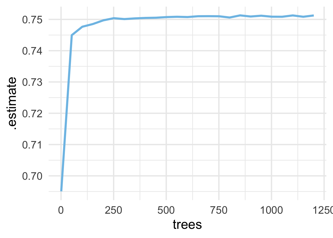
ggplot(test_n_trees, aes(trees, .estimate)) +
  geom_line()

And as we can see, we’re actually pretty safe with a much lower value, perhaps even as low as 100. However, because the models run very fast, we won’t worry about this too much. When we conduct our model tuning, we’ll drop to 500 trees instead of 1000 (still well above what it appears is needed).

Let’s see if we can improve performance by changing the mtry or min_n. Because we only have five predictor variables in this case, we don’t have a huge range to evaluate with mtry. But let’s setup a regular grid looking at values of 2, 3, 4 and 5 for mtry, and min_n values of 2, 5, 10, 15, 20, and 25.

grid <- expand.grid(mtry = 2:5,
                    min_n = c(2, seq(5, 25, 5)))

We can then use our fit_rf() function again, but this time setting the number of trees and looping through each of our mtry and min_n values.

The code below took about 18 and a half minutes to run on a local computer.

rf_tune <- map2_df(grid$mtry, grid$min_n, ~fit_rf(500, .x, .y))

rf_tune %>% 
  arrange(desc(.estimate))

## # A tibble: 24 x 6
##    .metric .estimator .estimate trees  mtry min_n
##    <chr>   <chr>          <dbl> <dbl> <int> <dbl>
##  1 roc_auc hand_till      0.752   500     2    25
##  2 roc_auc hand_till      0.752   500     2    15
##  3 roc_auc hand_till      0.752   500     2    20
##  4 roc_auc hand_till      0.752   500     2    10
##  5 roc_auc hand_till      0.751   500     2     5
##  6 roc_auc hand_till      0.751   500     2     2
##  7 roc_auc hand_till      0.749   500     3    25
##  8 roc_auc hand_till      0.748   500     3    20
##  9 roc_auc hand_till      0.745   500     3    15
## 10 roc_auc hand_till      0.744   500     4    25
## # … with 14 more rows

And notice that all of our top models here include our maximum number of predictors. So in this case, bagged trees are actually looking like our best option (rather than a random forest).

34.2.1.2 A regression example

For completeness, let’s run through another example using our statewide testing data. We didn’t use these data when fitting a bagged tree model, but we can start with a random forest anyway and see if it simplifies to a bagged tree.

First, let’s read in the data and create our testing set. We’ll only sample 20% of the data so things run more quickly.

state_tests <- get_data("state-test") %>% 
  select(-classification) %>% 
  slice_sample(prop = 0.2)

splt_reg <- initial_split(state_tests)
train_reg <- training(splt_reg)

Now we’ll create a recipe for these data. It is a bit more complicated than the last example because the data are a fair amount more complicated. The recipe looks like this:

rec_reg <- recipe(score ~ ., data = train_reg)  %>% 
  step_mutate(tst_dt = lubridate::mdy_hms(tst_dt),
              time_index = as.numeric(tst_dt)) %>%
  update_role(tst_dt, new_role = "time_index")  %>% 
  update_role(contains("id"), ncessch, new_role = "id vars")  %>% 
  step_novel(all_nominal())  %>% 
  step_unknown(all_nominal())  %>% 
  step_rollimpute(all_numeric(), -all_outcomes(), -has_role("id vars"))  %>% 
  step_medianimpute(all_numeric(), -all_outcomes(), -has_role("id vars"))  %>% # neccessary when date is NA
  step_zv(all_predictors())

The recipe above does the following

Defines score as the outcome and all other variables as predictors
Changes the tst_dt column (date the assessment was taken) to be a date (rather than character) and creates a new column that is a numeric version of the date
Changes the role of tst_dt from a predictor to a time_index, which is a special role that can be used to calculate date windows
Changes the role of all ID variables to an arbitrary "id vars" role, just so they are not used as predictors in the model
Recodes nominal columns such that previously unencountered levels of the variable will be recoded to a "new" level
Imputes an "unknown" category for all nominal data
Uses a rolling time window imputation (median for the closes 5 data points) to impute all numeric columns
In cases where the time window is missing, imputes with the median of the column for all numeric columns
Removes zero variance predictors

Next, we want to process the data using this recipe. Note that after we bake() the data, we remove those variables that are not predictors. Note that it might be worth considering keeping a categorical version of the school ID in the model (given that the school in which a student is enrolled is likely related to their score), but to keep things simple we’ll just remove all ID variables for now.

processed_reg <- rec_reg %>% 
  prep() %>% 
  bake(new_data = NULL) %>% 
  select(-contains("id"), -ncessch, -tst_dt)

processed_reg

## # A tibble: 28,414 x 32
##    gndr  ethnic_cd enrl_grd tst_bnch migrant_ed_fg ind_ed_fg sp_ed_fg tag_ed_fg
##    <fct> <fct>        <dbl> <fct>    <fct>         <fct>     <fct>    <fct>    
##  1 M     H                6 G6       N             N         N        N        
##  2 M     W                7 G7       N             N         N        Y        
##  3 M     W                8 3B       N             N         N        N        
##  4 F     W                7 G7       N             N         N        N        
##  5 M     H                5 2B       N             N         Y        N        
##  6 F     W                3 1B       N             N         Y        N        
##  7 F     W                8 3B       N             N         N        N        
##  8 M     M                6 G6       N             N         N        N        
##  9 M     H                7 G7       N             N         N        N        
## 10 M     H                7 G7       N             N         Y        N        
## # … with 28,404 more rows, and 24 more variables: econ_dsvntg <fct>,
## #   ayp_lep <fct>, stay_in_dist <fct>, stay_in_schl <fct>, dist_sped <fct>,
## #   trgt_assist_fg <fct>, ayp_dist_partic <fct>, ayp_schl_partic <fct>,
## #   ayp_dist_prfrm <fct>, ayp_schl_prfrm <fct>, rc_dist_partic <fct>,
## #   rc_schl_partic <fct>, rc_dist_prfrm <fct>, rc_schl_prfrm <fct>,
## #   lang_cd <fct>, tst_atmpt_fg <fct>, grp_rpt_dist_partic <fct>,
## #   grp_rpt_schl_partic <fct>, grp_rpt_dist_prfrm <fct>,
## #   grp_rpt_schl_prfrm <fct>, lat <dbl>, lon <dbl>, score <dbl>,
## #   time_index <dbl>

We’ll now use the processed data to fit a random forest, evaluating our model using the OOB samples. Let’s start by writing a function that fits the model for a given set of hyperparameters and returns a data frame with the hyperparameter values, our performance metric (RMSE) and the model object. Notice I’ve set num.threads = 16 because the local computer I’m working has (surprise!) 16 cores.

rf_fit_reg <- function(tree_n, mtry, min_n) {
  rf_mod_reg <- rand_forest() %>% 
    set_mode("regression") %>% 
    set_engine("ranger") %>% 
    set_args(mtry = mtry,
             min_n = min_n,
             trees = tree_n,
             num.threads = 16)

  rf_fit <- fit(rf_mod_reg, 
                formula = score ~ .,
                data = processed_reg)
  
  # output RMSE
  tibble(rmse = sqrt(rf_fit$fit$prediction.error)) %>% 
    mutate(trees = tree_n, 
           mtry = mtry, 
           min_n = min_n)
}

In the above I’ve used sqrt(rf_fit$fit$prediction.error) for the root mean square error, rather than using the model predictions with a {yardstick} function. This is because the default OOB error for a regression models with {ranger} is the mean square error, so we don’t have to do any predictions on our own - we just need to take the square root of this value. Most of the rest of this function is the same as before.

Let’s now conduct our tuning. First, let’s check how many predictors we have:

ncol(processed_reg) - 1

## [1] 31

Remember, for regression problems, a good place to start is around $m/3$, or 10.33. Let’s make a grid of mtry values, centered around 10.33. For min_n, we’ll use the same values we did before: 2, 5, 10, 15, 20, and 25. We’ll then evaluate the OOB RMSE across these different values and see if we need to conduct any more hyperparameter tuning.

grid_reg <- expand.grid(mtry = 5:15,
                        min_n = c(2, seq(5, 25, 5)))

And now we’ll use our function from above to fit each of these models, evaluating each with the OOB RMSE. We’ll start out with 1000 trees, then inspect that with our finalized model to make sure it is sufficient. Note that, even with using the OOB samples for our tuning, the following code takes a decent amount of time to run.

The code below took about 8 and half minutes to run on a local computer.

rf_reg_fits <- map2_df(grid_reg$mtry, grid_reg$min_n, 
                       ~rf_fit_reg(1000, .x, .y))

rf_reg_fits %>% 
  arrange(rmse)

rf_reg_fits <- readRDS(here::here("models", "random-forests", "rf_reg_fits.Rds"))

rf_reg_fits %>% 
  arrange(rmse)

## # A tibble: 66 x 4
##     rmse trees  mtry min_n
##    <dbl> <dbl> <int> <dbl>
##  1  86.1  1000     9    25
##  2  86.1  1000     9    20
##  3  86.2  1000     8    25
##  4  86.2  1000     8    20
##  5  86.2  1000     8    15
##  6  86.2  1000     7    15
##  7  86.2  1000     7    20
##  8  86.2  1000     7    25
##  9  86.2  1000    10    25
## 10  86.2  1000     7    10
## # … with 56 more rows

Let’s evaluate the hyperparameters we searched by plotting the mtry values against the RMSE, faceting by min_n.

ggplot(rf_reg_fits, aes(mtry, rmse)) +
  geom_line() +
  facet_wrap(~min_n)

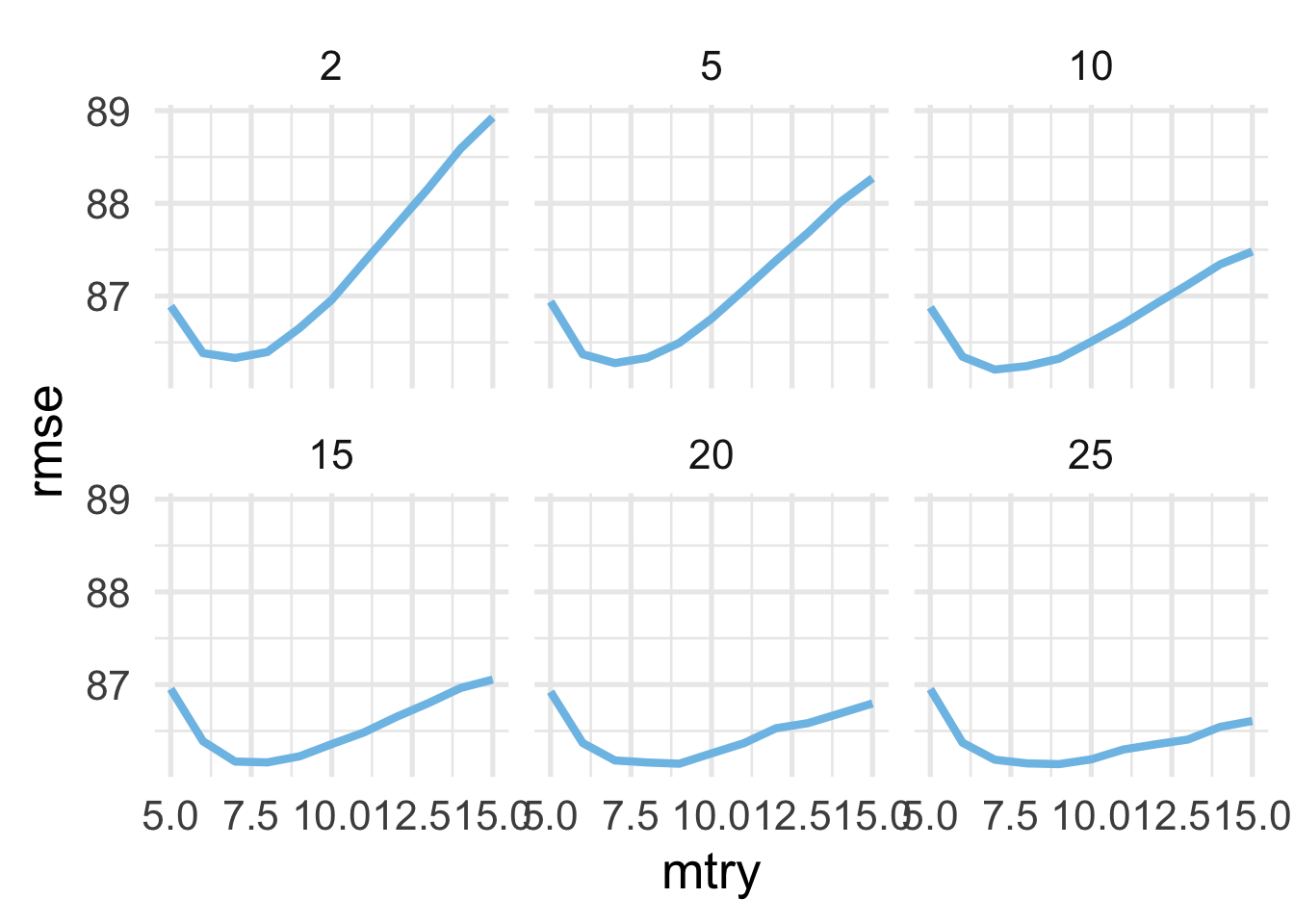
It looks like values of 7 or 8 are optimal for mtry, and our min_n is likely somewhere north of 20. Let’s see if we can improve performance more by tuning a bit more on min_n. We’ll evaluate values from 21 to 31 in increments of 2, while using both mtry values of 7 and 8.

grid_reg2 <- expand.grid(mtry = c(7, 8),
                         min_n = seq(21, 31, 2))

tic()
rf_reg_fits2 <- map2_df(grid_reg2$mtry, grid_reg2$min_n, 
                       ~rf_fit_reg(1000, .x, .y))
toc()

## 355.605 sec elapsed

rf_reg_fits2 <- rf_reg_fits2 %>% 
  arrange(rmse)
rf_reg_fits2

## # A tibble: 12 x 4
##     rmse trees  mtry min_n
##    <dbl> <dbl> <dbl> <dbl>
##  1  86.6  1000     8    31
##  2  86.6  1000     8    21
##  3  86.6  1000     8    29
##  4  86.6  1000     8    25
##  5  86.6  1000     8    23
##  6  86.6  1000     8    27
##  7  86.6  1000     7    23
##  8  86.6  1000     7    21
##  9  86.6  1000     7    31
## 10  86.7  1000     7    25
## 11  86.7  1000     7    29
## 12  86.7  1000     7    27

Notice the RMSE is essentially equivalent for all models listed above. We’ll go forward with the first model, but any of these combinations of hyperparameters likely provide similar out-of-sample predictive accuracy (according to RMSE).

Finally, before moving on to evaluating our model against the test set, we would likely want to make sure that we fit the model with a sufficiently large number of trees. Let’s investigate with a model that had the lowest RMSE. We’ll use trees from 500 to 1500 by increments of 100.

tic()
rf_reg_ntrees <- map_df(seq(500, 1500, 100), 
                        ~rf_fit_reg(.x, 
                                    mtry = rf_reg_fits2$mtry[1], 
                                    min_n = rf_reg_fits2$min_n[1])
                        )
toc()

## 288.102 sec elapsed

And now we’ll plot the number of trees against the RMSE, looking for a point of stability.

ggplot(rf_reg_ntrees, aes(trees, rmse)) +
  geom_line()

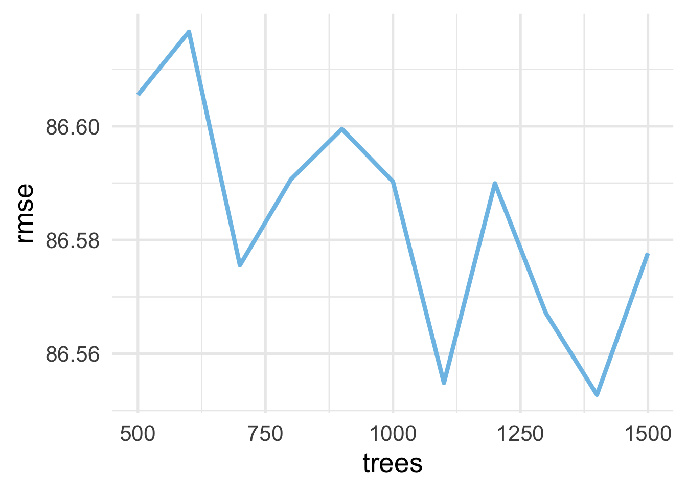
Hmm… that doesn’t look terrifically stable. BUT WAIT! Notice the bottom to the top of the y-axis is only about one-tenth of a point difference. So really, this is not a problem with instability, but that it is actually stable across all these values. Just to prove this to ourselves, let’s look at the same plot, but making the y-axis span one point (which is still not very much), going from 86 to 87.

ggplot(rf_reg_ntrees, aes(trees, rmse)) +
  geom_line() +
  ylim(86, 87)

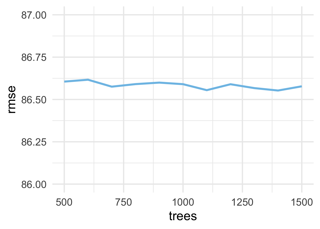
And now it looks more stable. So even with 500 trees we likely would have been fine.

From here, we could continue on to evaluate our final model against the test set using the last_fit() function, but we will leave that as an exercise for the reader. Note that we also only worked with 5% of the total data. The hyperparameters that we settled on may be different if we used more of the data. We could also likely improve performance more by including additional information in the model - e.g., information on staffing and funding, the size of the school or district, indicators of the economic and demographic makeup of the surrounding area, or practices related to school functioning (e.g., use of suspension/expulsion).

34.3 Feature and model interpretation

A considerable benefit of decision tree models is that they are relatively easy to understand, in terms of how predictions are made. It’s perhaps less clear why specific splits have been made, but it’s relatively straightforward to communicate with stakeholders how predictions are made. This is because the tree itself can be followed, like a road map, to the terminal node. The tree is just a series of if/then statements. Unfortunately, this ease of interpretation all goes out the window with bagged trees and random forests. Instead of just building one decision tree, we are building hundreds or even thousands, with each tree (or at least most trees) being at least slightly different. So how do we communicate the results of our model with stakeholders? How can we effectively convey how our model makes predictions?

Perhaps the most straightforward way to communicate complex models with stakeholders is to focus on feature importance. That is, which features in the model are most important in establishing the prediction. We can do this with {ranger} models using the {vip} package (vip stands for variable importance plots).

In a standard decision, a variable is selected at a given node if it improves the objective function score. The relative importance of a given variable is then determined by the sum of the squared improvements (see {vip} documentation). This basic idea is extended to ensembles of trees, like bagged trees and random forest, by computing the mean of these importance scores across all trees in the ensemble.

To obtain variable importance scores, we first have to re-run our {ranger} model, requesting it computes variable importance metrics. We do this by specifying importance = "impurity" (which is the Gini index for classification problems).

# specify the model and request a variable importance metric
rf_mod_reg_final <- rand_forest() %>% 
    set_mode("regression") %>% 
    set_engine("ranger") %>% 
    set_args(mtry = rf_reg_fits2$mtry[1],
             min_n = rf_reg_fits2$min_n[1],
             trees = 1000,
             importance = "impurity")

# fit the model
tic()
rf_fit_reg_final <- fit(rf_mod_reg_final,
                        score ~ .,
                        processed_reg)
toc()

## 61.319 sec elapsed

And now we can request variable importance scores with vip::vi(), or a variable importance plot with vip::vip(). Let’s first look at the scores.

library(vip)
vi(rf_fit_reg_final$fit)

## # A tibble: 31 x 2
##    Variable    Importance
##    <chr>            <dbl>
##  1 enrl_grd     33742487.
##  2 tag_ed_fg    31287898.
##  3 sp_ed_fg     29788749.
##  4 econ_dsvntg  28709267.
##  5 tst_bnch     16228993.
##  6 ayp_lep      15274675.
##  7 lon          14849760.
##  8 lat          14241044.
##  9 time_index   12172779.
## 10 ethnic_cd    10888929.
## # … with 21 more rows

The results of this investigation are not entirely surprising. The enrl_grd the student in is the most important predictor of their score. Following grade level, the students’ economic disadvantaged status is the most predictive feature in the model, following a long history of evidence documenting differential achievement by socioeconomic status. Students classified as talented and gifted (TAG), and those who received special education services are the next two most predictive variables, followed by the physical location of the school (lat = latitude and lon = longitude). Each of these variables would be among those that we might have guessed, a priori, would be the most predictive.

Let’s look at a plot showing the relative importance of the features in our model.

vip(rf_fit_reg_final$fit)

Our inferences here are similar, but this view helps us see more clearly that the first three variables are similarly important, then there is a bit of a dip for with special education status, followed by a sizeable dip for latitude and longitude. The tst_bnch feature is essentially a categorical version of grade level (so we are modeling it as both a continuous and categorical feature; the merits of such an approach could be argued, but we see that we are getting improvements from both versions).

With bagged trees and random forests, we can also look at variable importance in a slightly different way. Rather than summing the contributions for each tree, and taking the average across trees, we can compute the OOB error for a given tree, then shuffle the values for a given variable and re-compute the OOB error. If the variable is important, the OOB error will increase as we perturb the given variable, but otherwise the error will stay (approximately) the same (see Wright, Ziegler, and König, 2016).

To get this purmutation-based importance measure, we just change importance to "purmutation". Let’s do this and see if the resulting plot differs.

rf_mod_reg_final2 <- rand_forest() %>% 
    set_mode("regression") %>% 
    set_engine("ranger") %>% 
    set_args(mtry = rf_reg_fits2$mtry[1],
             min_n = rf_reg_fits2$min_n[1],
             trees = 1000,
             importance = "purmutation")

tic()
rf_fit_reg_final2 <- fit(rf_mod_reg_final,
                        score ~ .,
                        processed_reg)
toc()

## 69.49 sec elapsed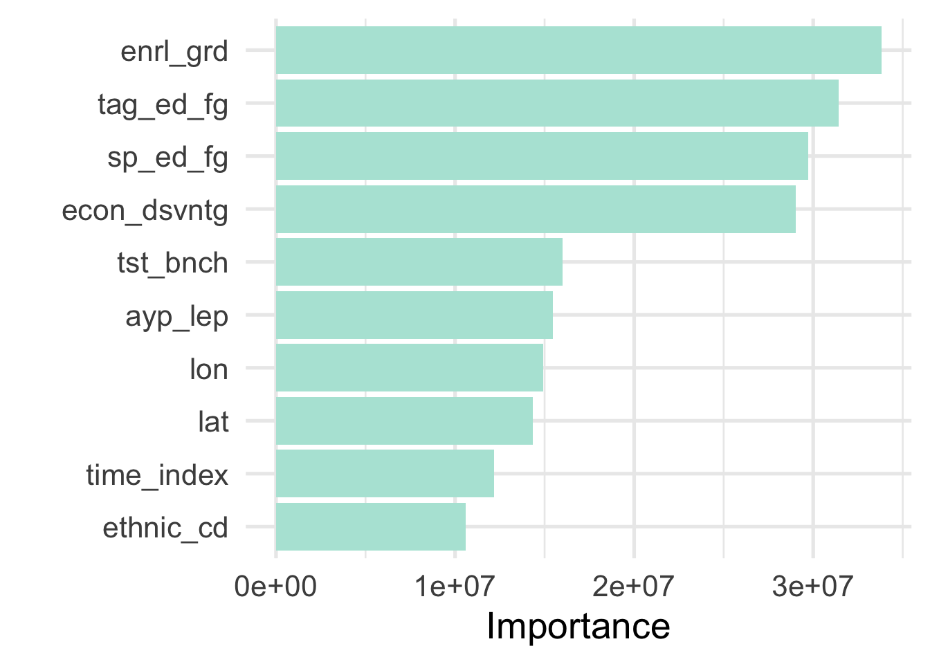

vip(rf_fit_reg_final2$fit)

As we can see, there are a few small differences, but generally the results agree, providing us with greater confidence in the ordering variable importance. If the results did not generally align that may be evidence that our model is unstable and we would likely want to probe our model a bit more.

Inspecting variable importance helps us understand which variables contribute to our model predictions, but not necessarily how they relate to the outcome. For that, we can look at partial dependency plots via the {pdp} package (which is developed by the same people who created {vip}).

Partial dependency plots show the marginal effect of a feature on the outcome. This can help us to understand the directionality of the effect and whether it is generally linear or not. For example, we would probably expect that students’ scores would increase roughly linearly and monotonically with enrl_grd. To see if that’s the case we case we use the pdp::partial() function. Note that these functions take a bit of time to run, as shown by the timings

library(pdp)
partial(rf_fit_reg_final$fit, 
        pred.var = "enrl_grd",
        train = processed_reg,
        plot = TRUE,
        plot.engine = "ggplot2")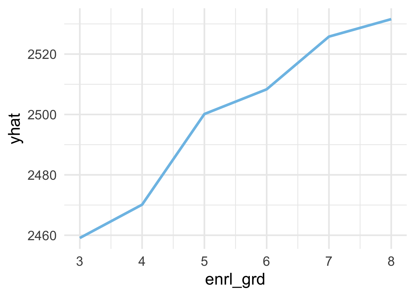

And we can see that, yes, the relation is roughly linear and monotonically increasing.

What if we want to explore more than one variable? Let’s look at the geographic location of the school. The code below takes a bit of time to run (~30 minutes on a local computer). Additionally, while we could just add plot = TRUE and plot.engine = "ggplot2", we’ve saved the object and plotted it separately to have a bit more control over how the plot is rendered.

The code below took about 30 minutes to run on a local computer.

partial_lon_lat <- partial(rf_fit_reg_final$fit, 
        pred.var = c("lon", "lat"),
        train = processed_reg)

ggplot(partial_lon_lat, aes(lon, lat)) +
  geom_tile(aes(fill = yhat)) +
  coord_map() +
  theme_void() +
  theme(legend.position = "bottom",
        legend.key.width = unit(1, "cm"))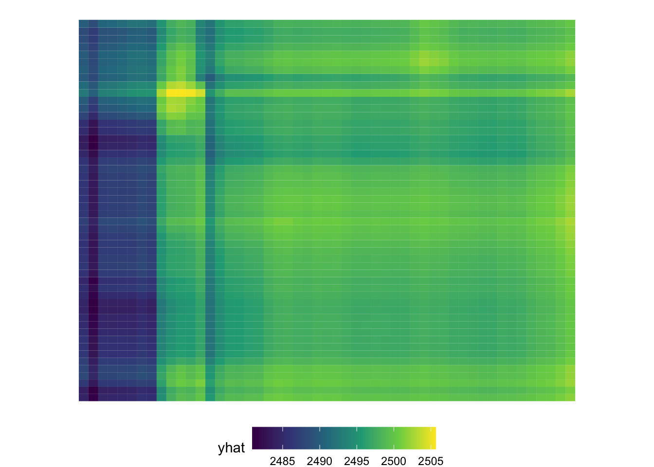

Because this is geographic data, and we know the data come from Oregon (although they are simulated) we can interpret this as if we were looking at a physical map. One notable aspect is that there is a fairly clear band running north/south in the western part of the state. This is roughly where I-5 runs and where many of the more populous towns/cities are located, including Ashland/Medford in the south, Eugene around the center, and Portland in the north. We could even overlay an image of Oregon here, which actually helps us with interpretation a bit more.

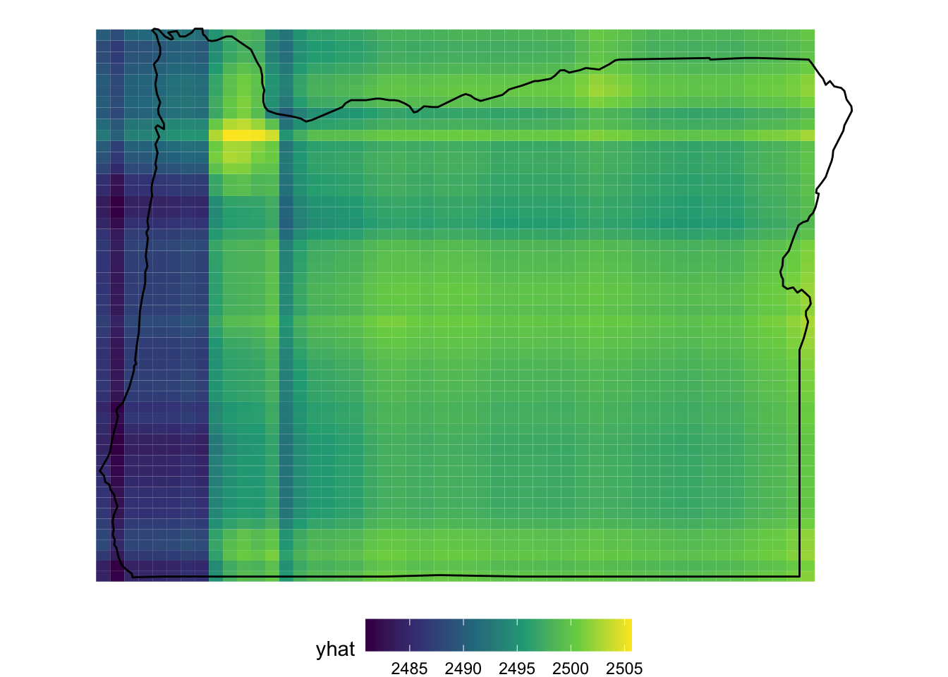
Note that, when the PDP is created, it just creates a grid for prediction. So when we overlay the map of Oregon, we see some areas where the prediction extends outside of the state, which are not particularly trustworthy.

Finally, we might also be interested in the individual variability of a feature. Let’s again look at the enrolled grade of students. In this case, we’ll create individual conditional expectation plots, or ICE curves, which are equivalent to PDP’s but for individual observations. The {pdp} package can again create these for us. The process for creating them is essentially equivalent, but we provide one additional argument, ice = TRUE. Note that we can use plot = TRUE here too but I’ve just output the values to have a bit more control of how the plot renders.

ice_grade <- partial(rf_fit_reg_final$fit, 
                     pred.var = "enrl_grd",
                     train = processed_reg,
                     ice = TRUE)

ggplot(ice_grade, aes(enrl_grd, yhat)) +
  geom_line(aes(group = yhat.id),
            color = "gray40",
            size = 0.1,
            alpha = 0.1) +
  stat_summary(geom = "line", fun = "mean")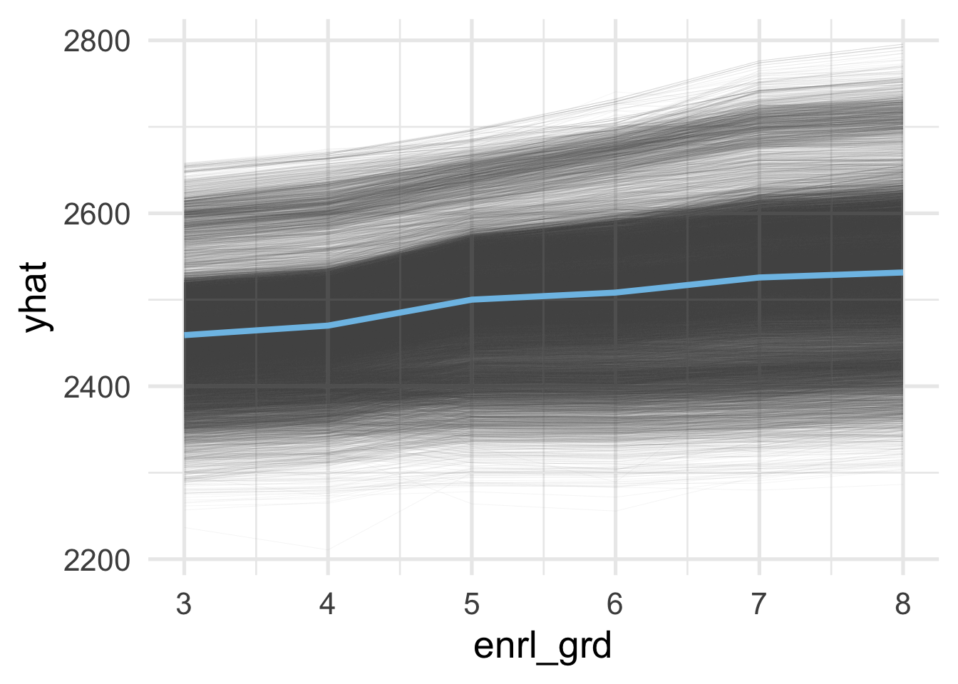

And as we would likely expect, there is a lot of variation here in expected scores across grades.

Bagged trees can often lead to better predictions than a single decision tree by creating ensembles of trees based on bootstrap resamples of the data and aggregating the results across all trees. Random forests extend this framework by randomly sampling $m$ columns at each split of each tree that is grown in the ensemble (or forest) which can help decorrelate the trees and, often, lead to better overall predictions. Unfortunately creating an ensemble of trees also makes feature and model interpretation a bit more difficult. Tools like variable importance and partial dependence plots can be an efficient means of communicating how and why a model is making the predictions it is, while still maintaining strong overall model performance. For more information on these and other methods, see Molnar, 2020.